4. Keyframes
4.1. Inverse Depth Update
To be added
4.2. Immature Point Activation
To be added
4.3. Sliding Window Optimization
4.3.1. Error Function Formulation

If a specific frame is determined as a keyframe, the error function must be updated between keyframes within the sliding window and a new keyframe. At this time, Local Bundle Adjustment (LBA) is performed to optimize not only the keyframe but also the points on the map connected to it.
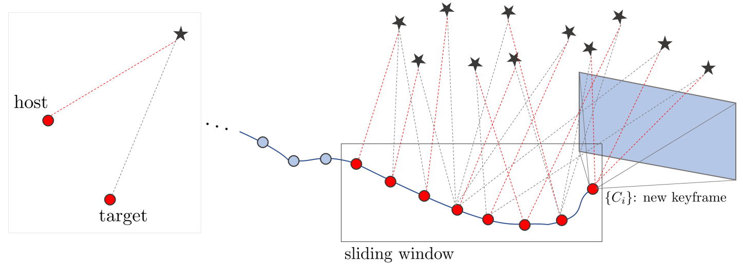
Note that one map point is optimized by connecting it with two keyframes (host, target). Here, the host keyframe is the keyframe in which the corresponding map point is found first, and the target keyframe is the keyframe found later.

Also, to reduce the amount of computation in the optimization process, Jacobian $\frac{\partial \mathbf{r}}{\partial \xi_{th}}$ calculated based on the relative pose between the host and target keyframes is used instead of Jacobian $\frac{\partial \mathbf{r}}{\partial \xi_{wh}},\frac{\partial \mathbf{r}}{\partial \xi_{wt}}$ calculated based on the world coordinate system of the camera when calculating the Jacobian. Therefore, Adjoint Transformation is used to optimize the camera pose $\mathbf{T}_{wh}, \mathbf{T}_{wt}$ based on the world coordinate system of the two keyframes using the Jacobian. (explained in a later section)
In order to perform sliding window optimization, an error function must first be set. At this time, the parameters of the error function are pose(6) + photometric(2) + camera intrinsic(4) + idepth(N), and a total of 12+N parameters are used for optimization. For reference, in the initialization process, 8+N parameters were optimized except for camera intrinsic (4). That is, except for the camera intrinsics ($(f_{x}, f_{y}, c_{x}, c_{y})$), the Jacobian is the same as before.

The error (residual) can be set as follows.
$$\mathbf{r} = \mathbf{I}_{t}(\mathbf{p}_{t}) - \exp(a)( \mathbf{I}_{h}(\mathbf{p}_{h}) - b_{0}) - b$$
- $\mathbf{p}_{t} = \pi(\exp(\xi^{\wedge}_{th})\mathbf{X}_{1}) = \pi(\exp(\xi^{\wedge}_{th})\pi^{-1}(\mathbf{p}_{h}))$
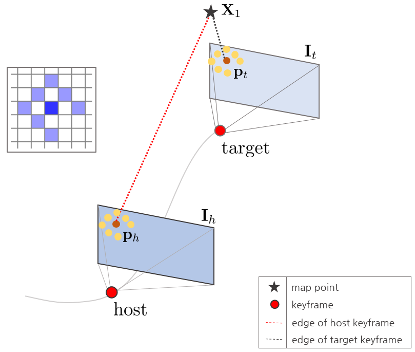
At this time, the residual means the error sum of 8-point patch points rather than one point. Finally, the error function applied to the huber norm is as follows.
$$\text{H}(\mathbf{r}) = w_{h}\mathbf{r}^{2}$$
In order to find the parameter for which the error function is minimized, the problem of minimizing the $f(\mathbf{x})$ that satisfies $f(\mathbf{x})^{T}f(\mathbf{x}) = \text{H}(\mathbf{r})$ is changed to the following.
$$f(\mathbf{x}) = \sqrt{w_{h}} \ \mathbf{r} = \sqrt{w_{h}}(\mathbf{I}_{2}(\mathbf{p}_{2}) - \exp(a)(\mathbf{I}_{1}(\mathbf{p}_{1}-b_{0})) - b)$$
The state variable $\mathbf{x}$ in the error function $f(\mathbf{x})$ is
$$f(\mathbf{x}) = \sqrt{w_{h}} \ \mathbf{r} = \sqrt{w_{h}}(\mathbf{I}_{t}(\mathbf{p}_{t}) - \exp(a)(\mathbf{I}_{h}(\mathbf{p}_{h}-b_{0})) - b)$$
$$\mathbf{x} = [ \ \rho^{(1)}_{1}, \cdots, \rho^{(N)}_{1}, \delta \xi^{T}, a, b, \mathbf{c} \ ]^{T}_{(N+12) \times 1}$$
- $\rho_{1}^{(i)}$ : i-th inverse depth value in image 1 (N)
- $\delta \xi$ : Relative pose change between two cameras (twist) (6-dimensional vector) (6)
- $a,b$: Parameters that adjust the image brightness considering the exposure time between the two images (2)
- $\mathbf{c}$ : camera internal parameters (fx,fy,cx,cy) (4)
Unlike the initialization process, it can be seen that the error function $\mathbf{x}$ includes the camera intrinsic $\mathbf{c}$. In the initialization process, Jacobians necessary for optimization were already derived as follows.
idepth(N)
$$\frac{\partial f(\mathbf{x})}{\partial \rho_{1}} = \sqrt{w_{h}}\rho_{1}^{-1}\rho_{2}(\nabla \mathbf{I}_{x}f_{x}(t_{x}-u_{2}^{'}t_{z}) + \nabla \mathbf{I}_{y}f_{y}(t_{y} - v_{2}^{'}t_{z}))$$
pose(6)
$$\frac{\partial f(\mathbf{x})}{\partial \delta \xi} =\sqrt{w_{h}}
\begin{bmatrix}
\nabla \mathbf{I}_{x}\rho_{2}f_{x} \\
\nabla \mathbf{I}_{y}\rho_{2}f_{y} \\
-\rho_{2}(\nabla \mathbf{I}_{x}f_{x}u_{2}^{'} + \nabla \mathbf{I}_{y}f_{y}v_{2}^{'}) \\
-\nabla \mathbf{I}_{x}f_{x}u_{2}^{'}v_{2}^{'} -\nabla \mathbf{I}_{y}f_{y}(1+v_{2}^{'2}) \\
\nabla \mathbf{I}_{x}f_{x}(1+u_{2}^{'2}) + \nabla \mathbf{I}_{y}f_{y}u_{2}^{'}v_{2}^{'} \\
-\nabla \mathbf{I}_{x}f_{x}v_{2}^{'} + \nabla \mathbf{I}_{y}f_{y}u_{2}^{'}\\
\end{bmatrix}^{T}$$
photometric(2)
$$\frac{\partial f(\mathbf{x})}{\partial a} = - \sqrt{w_{h}} \exp(a)\mathbf{I}_{1}(\mathbf{p}_{1})$$
$$\frac{\partial f(\mathbf{x})}{\partial b} = - \sqrt{w_{h}}$$
However, in the sliding window optimization process, Jacobian of Camera Intrinsic $\frac{\partial f(\mathbf{x})}{\partial \mathbf{c}}$ must be derived additionally.
4.3.2. Derivate Jacobian of Camera Intrinsics

$\frac{\partial f(\mathbf{x})}{\partial \mathbf{c}}$ can be decomposed as follows.
$$\frac{\partial f(\mathbf{x})}{\partial \mathbf{c}}
=
\frac{\partial f(\mathbf{x})}{\partial \mathbf{p}_{t}}
\frac{\partial \mathbf{p}_{t}}{\partial \mathbf{c}}
$$
At this time, since $f(\mathbf{x}) = \sqrt{w_{h}} \ \mathbf{r}$, it is simply expressed as a residual term as follows.
$$\frac{\partial \mathbf{r}}{\partial \mathbf{c}}
=
\frac{\partial \mathbf{r}}{\partial \mathbf{p}_{t}}
\frac{\partial \mathbf{p}_{t}}{\partial \mathbf{c}}
$$
$\frac{\partial \mathbf{r}}{\partial \mathbf{p}_{t}}$ has already been derived as follows in the Initialization section.
$$\frac{\partial\mathbf{r}}{\partial \mathbf{p}_{t}} = \frac{\partial \mathbf{I_{t}}(\mathbf{p_{t}})}{\partial \mathbf{p}_{t}} = [ \ \nabla \mathbf{I}_{x} \ \ \nabla \mathbf{I}_{y} \ ]$$
And $\frac{\partial \mathbf{p}_{t}}{\partial \mathbf{c}}$ can be derived as follows.
\begin{equation*}
\begin{aligned}
\frac{\partial \mathbf{p}_{t}}{\partial \mathbf{c}}
&=
\begin{bmatrix}
\frac{\partial u_{t}}{\partial f_{x}} & \frac{\partial u_{t}}{\partial f_{y}}
& \frac{\partial u_{t}}{\partial c_{x}}
& \frac{\partial u_{t}}{\partial c_{y}}
\\
\frac{\partial v_{t}}{\partial f_{x}} & \frac{\partial v_{t}}{\partial f_{y}}
& \frac{\partial v_{t}}{\partial c_{x}}
& \frac{\partial v_{t}}{\partial c_{y}}
\end{bmatrix} \\
&=
\begin{bmatrix}
\bar{u}_{t} + f_{x}\frac{\partial \bar{u}_{t}}{\partial f_{x}}
& f_{x}\frac{\partial \bar{u}_{t}}{\partial f_{y}}
& f_{x}\frac{\partial \bar{u}_{t}}{\partial c_{x}} + 1
& f_{x}\frac{\partial \bar{u}_{t}}{\partial c_{y}}
\\
f_{y}\frac{\partial \bar{v}_{t}}{\partial f_{x}}
& \bar{v}_{t} + f_{y}\frac{\partial \bar{v}_{t}}{\partial f_{y}}
& f_{y}\frac{\partial \bar{v}_{t}}{\partial c_{x}}
& f_{y}\frac{\partial \bar{v}_{t}}{\partial c_{y}}+1
\end{bmatrix}
\end{aligned}
\end{equation*}
\begin{equation*}
\begin{aligned}
\because
u_{t} = f_{x}\bar{u}_{t} + c_{x} \\
v_{t} = f_{y}\bar{v}_{t} + c_{y}
\end{aligned}
\end{equation*}
Next, we need to find the value below. \begin{equation*}
\begin{aligned}
\begin{bmatrix}
\frac{\partial \bar{u}_{t}}{\partial f_{x}} & \frac{\partial \bar{u}_{t}}{\partial f_{y}}
& \frac{\partial \bar{u}_{t}}{\partial c_{x}}
& \frac{\partial \bar{u}_{t}}{\partial c_{y}} \\
\frac{\partial \bar{v}_{t}}{\partial f_{x}} & \frac{\partial \bar{v}_{t}}{\partial f_{y}}
& \frac{\partial \bar{v}_{t}}{\partial c_{x}}
& \frac{\partial \bar{v}_{t}}{\partial c_{y}}
\end{bmatrix}
\end{aligned}
\end{equation*}. First, expanding the equation is like: \begin{equation*}
\begin{aligned}
\begin{bmatrix}
\bar{u}_{t} & \bar{v}_{t} & 1 \end{bmatrix}
\end{aligned}
\end{equation*}
\begin{equation*}
\begin{aligned}
\begin{bmatrix}
\bar{u}_{t} & \bar{v}_{t} & 1 \end{bmatrix}^{T}
&=
\rho_{t}(\mathbf{R}\mathbf{X}_{1} + \mathbf{t})\\
&=
\rho_{t}(\rho_{h}^{-1}\mathbf{R}\mathbf{K}^{-1}\mathbf{p}_{h} + \mathbf{t}) \\
&=
\rho_{t}\rho_{h}^{-1}(\mathbf{R}\mathbf{K}^{-1}\mathbf{p}_{h}) + \rho_{t}\mathbf{t} \\
&=
\rho_{t}\rho_{h}^{-1}
\begin{bmatrix}
& & \\
& \mathbf{R} & \\
& &
\end{bmatrix}
\begin{bmatrix}
f_{x}^{-1}& & -f_{x}^{-1}c_{x}\\
& f_{y}^{-1} & -f_{y}^{-1}c_{y} \\
& & 1
\end{bmatrix}
\begin{bmatrix}
u_{h} \\ v_{h} \\ 1
\end{bmatrix}
+
\rho_{t}
\begin{bmatrix}
t_{x} \\ t_{y} \\ t_{z}
\end{bmatrix} \\
&=
\rho_{t}\rho_{h}^{-1}
\begin{bmatrix}
& & \\
& \mathbf{R} & \\
& &
\end{bmatrix}
\begin{bmatrix}
f_{x}^{-1}(u_{h}-c_{x}) \\
f_{y}^{-1}(v_{h}-c_{y}) \\
1
\end{bmatrix}
+
\rho_{t}
\begin{bmatrix}
t_{x} \\ t_{y} \\ t_{z}
\end{bmatrix} \\
&=
\rho_{t}\rho_{h}^{-1}
\begin{bmatrix}
r_{11}f_{x}^{-1}(u_{h}-c_{x}) + r_{12}f_{y}^{-1}(v_{h}-c_{y}) + r_{13} \\
r_{21}f_{x}^{-1}(u_{h}-c_{x}) + r_{22}f_{y}^{-1}(v_{h}-c_{y}) + r_{23} \\
r_{31}f_{x}^{-1}(u_{h}-c_{x}) + r_{32}f_{y}^{-1}(v_{h}-c_{y}) + r_{33}
\end{bmatrix}
+
\rho_{t}
\begin{bmatrix}
t_{x} \\ t_{y} \\ t_{z}
\end{bmatrix} \\
\end{aligned}
\end{equation*}
Therefore, $\bar{u}_{t}$ and $\bar{v}_{t}$ can be expressed as follows.
$$\therefore
\bar{u}_{t} = \frac
{r_{11}f_{x}^{-1}(u_{h}-c_{x}) + r_{12}f_{y}^{-1}(v_{h}-c_{y}) + r_{13} + \rho_{h}t_{x}}
{r_{31}f_{x}^{-1}(u_{h}-c_{x}) + r_{32}f_{y}^{-1}(v_{h}-c_{y}) + r_{33} + \rho_{h}t_{z}}
$$
$$
\bar{v}_{t} = \frac
{r_{21}f_{x}^{-1}(u_{h}-c_{x}) + r_{22}f_{y}^{-1}(v_{h}-c_{y}) + r_{23} + \rho_{h}t_{y}}
{r_{31}f_{x}^{-1}(u_{h}-c_{x}) + r_{32}f_{y}^{-1}(v_{h}-c_{y}) + r_{33} + \rho_{h}t_{z}}
$$
Using the above formula, \begin{equation*}
\begin{aligned}
\begin{bmatrix}
\frac{\partial \bar{u}_{t}}{\partial f_{x}} & \frac{\partial \bar{u}_{t}}{\partial f_{y}}
& \frac{\partial \bar{u}_{t}}{\partial c_{x}}
& \frac{\partial \bar{u}_{t}}{\partial c_{y}} \\
\frac{\partial \bar{v}_{t}}{\partial f_{x}} & \frac{\partial \bar{v}_{t}}{\partial f_{y}}
& \frac{\partial \bar{v}_{t}}{\partial c_{x}}
& \frac{\partial \bar{v}_{t}}{\partial c_{y}}
\end{bmatrix}
\end{aligned}
\end{equation*} is obtained as follows.
$$\frac{\partial \bar{u}_{t}}{\partial f_{x}} = \rho_{t}\rho_{h}^{-1}(r_{31}\bar{u}_{t} - r_{11})f_{x}^{-2}(u_{h}-c_{x})$$
$$\frac{\partial \bar{u}_{t}}{\partial f_{y}} = \rho_{t}\rho_{h}^{-1}(r_{32}\bar{u}_{t} - r_{12})f_{y}^{-2}(v_{h}-c_{y})$$
$$\frac{\partial \bar{u}_{t}}{\partial c_{x}} = \rho_{t}\rho_{h}^{-1}(r_{31}\bar{u}_{t} - r_{11})f_{x}^{-1}$$
$$\frac{\partial \bar{u}_{t}}{\partial c_{y}} = \rho_{t}\rho_{h}^{-1}(r_{32}\bar{u}_{t} - r_{12})f_{y}^{-1}$$
$$\frac{\partial \bar{v}_{t}}{\partial f_{x}} = \rho_{t}\rho_{h}^{-1}(r_{31}\bar{v}_{t} - r_{21})f_{x}^{-2}(u_{h}-c_{x})$$
$$\frac{\partial \bar{v}_{t}}{\partial f_{y}} = \rho_{t}\rho_{h}^{-1}(r_{32}\bar{v}_{t} - r_{22})f_{y}^{-2}(v_{h}-c_{y})$$
$$\frac{\partial \bar{v}_{t}}{\partial c_{x}} = \rho_{t}\rho_{h}^{-1}(r_{31}\bar{v}_{t} - r_{21})f_{x}^{-1}$$
$$\frac{\partial \bar{u}_{t}}{\partial c_{y}} = \rho_{t}\rho_{h}^{-1}(r_{32}\bar{v}_{t} - r_{22})f_{y}^{-1}$$
Finally, $\frac{\partial \mathbf{p}_{t}}{\partial \mathbf{c}}$ can be expressed as:
Camera Intrinsic(4)
\begin{equation*}
\begin{aligned}
\frac{\partial \mathbf{p}_{t}}{\partial \mathbf{c}}
&=
\begin{bmatrix}
\frac{\partial u_{t}}{\partial f_{x}} & \frac{\partial u_{t}}{\partial f_{y}}
& \frac{\partial u_{t}}{\partial c_{x}}
& \frac{\partial u_{t}}{\partial c_{y}}
\\
\frac{\partial v_{t}}{\partial f_{x}} & \frac{\partial v_{t}}{\partial f_{y}}
& \frac{\partial v_{t}}{\partial c_{x}}
& \frac{\partial v_{t}}{\partial c_{y}}
\end{bmatrix} \\
&=
\begin{bmatrix}
\bar{u}_{t} + f_{x}\frac{\partial \bar{u}_{t}}{\partial f_{x}}
& f_{x}\frac{\partial \bar{u}_{t}}{\partial f_{y}}
& f_{x}\frac{\partial \bar{u}_{t}}{\partial c_{x}} + 1
& f_{x}\frac{\partial \bar{u}_{t}}{\partial c_{y}}
\\
f_{y}\frac{\partial \bar{v}_{t}}{\partial f_{x}}
& \bar{v}_{t} + f_{y}\frac{\partial \bar{v}_{t}}{\partial f_{y}}
& f_{y}\frac{\partial \bar{v}_{t}}{\partial c_{x}}
& f_{y}\frac{\partial \bar{v}_{t}}{\partial c_{y}}+1
\end{bmatrix} \\
&=
\begin{bmatrix}
\bar{u}_{t} + \rho_{t}\rho_{h}^{-1}f_{x}^{-1}(r_{31}\bar{u}_{t} - r_{11})(u_{h}-c_{x})&
\rho_{t}\rho_{h}^{-1}f_{x}f_{y}^{-2}(r_{32}\bar{u}_{t} - r_{12})(v_{h}-c_{y})&
\rho_{t}\rho_{h}^{-1}(r_{31}\bar{u}_{t} - r_{11}) + 1&
\rho_{t}\rho_{h}^{-1}f_{x}f_{y}^{-1}(r_{32}\bar{u}_{t} - r_{12})
\\
\rho_{t}\rho_{h}^{-1}f_{x}^{-2}f_{y}(r_{31}\bar{v}_{t} - r_{21})(u_{h}-c_{x})&
\bar{v}_{t} + \rho_{t}\rho_{h}^{-1}f_{y}^{-1}(r_{32}\bar{v}_{t} - r_{22})(v_{h}-c_{y})&
\rho_{t}\rho_{h}^{-1}f_{x}^{-1}f_{y}(r_{31}\bar{v}_{t} - r_{21})&
\rho_{t}\rho_{h}^{-1}(r_{32}\bar{u}_{t} - r_{12}) + 1
\end{bmatrix}
\end{aligned}
\end{equation*}
4.3.3. First Estimate Jacobian (FEJ)
When performing sliding window optimization, the state variable $\mathbf{x}$ is updated every iteration. At this time, the $\boxplus$ operator is an operator that updates N+12 states for each parameter.
$$\mathbf{x} \leftarrow \Delta \mathbf{x} \boxplus \mathbf{x}$$
- $\mathbf{x} = [ \ \rho^{(1)}_{1}, \cdots, \rho^{(N)}_{1}, \delta \xi^{T}, a, b, \mathbf{c} \ ]^{T}_{(N+12) \times 1}$
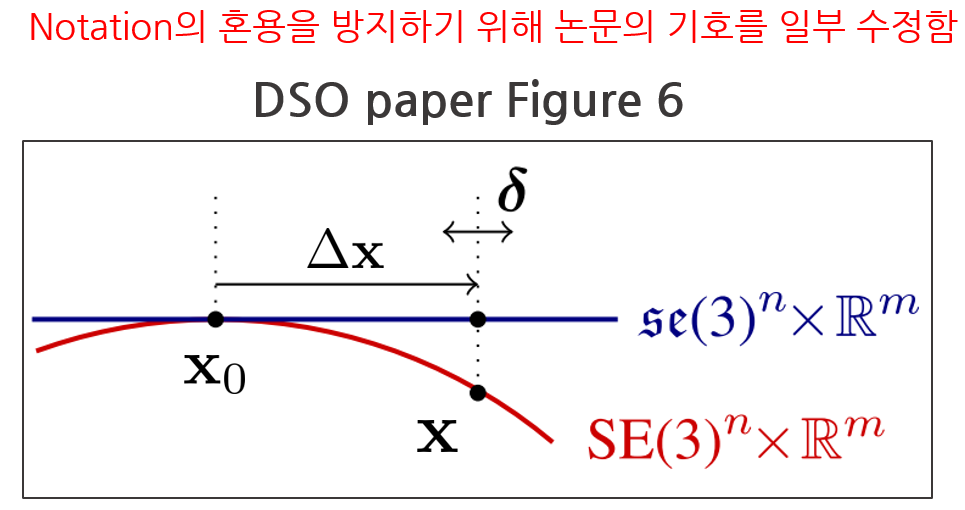
- $\mathbf{x}_{0}$ : state variable at the time of starting LBA
- $\mathbf{x}$ : state variable after LBA ends
- $\Delta \mathbf{x}$ : Cumulative increment due to each iteration update (including marginalization)
- $\delta$ : The incremental amount of each iteration update
Some of the symbols in the thesis were modified to prevent mixed use of notation. In DSO, optimization is performed 6 times each time LBA is performed. If the Jacobian is newly calculated for each iteration, the following disadvantages exist. (See https://blog.csdn.net/heyijia0327/article/details/53707261 for details)
1. Real-time performance cannot be guaranteed because the amount of computation is greatly increased.
2. When Jacobians of different states are used together in one system, there is a possibility of causing performance degradation.
Therefore, when performing LBA, even if the state variable $\mathbf{x}$ changes due to an update every iteration (include marginalization), the Jacobian is not calculated anew and the LBA starts at the point ($\mathbf{x}_{0} $) is called the First Estimate Jacobian (FEJ). The order of application of FEJ is as follows.
1. Before starting LBA, save the current $\mathbf{x}$ to $\mathbf{x}_{0}$ and calculate the Jacobian.
$$\mathbf{x}_{0} \leftarrow \mathbf{x}, \text{ compute } \mathbf{J}|_{\mathbf{x}_{0}}$$
2. Accumulate updated values at every iteration while performing LBA.
$$\Delta \mathbf{x}\leftarrow\Delta \mathbf{x}+\delta$$
3. During each iteration, the Jacobian uses the value calculated from $\mathbf{x}_{0}$.
4. When the LBA iteration is over, the incremental amount accumulated in the current state is updated.
$$\mathbf{x} \leftarrow \Delta \mathbf{x} \boxplus \mathbf{x}_{0}$$
4.3.4. Adjoint Transformation

As described above, in DSO, two keyframes (host, target) are connected to one map point. Accordingly, in order to reduce the amount of computation during optimization, Jacobian $\frac{\partial \mathbf{r}}{\partial \xi_{th}}$ calculated based on the relative pose between the target and host keyframes is used.
However, if an iterative solution is obtained using the Jacobian, only the relative pose between the two host and target keyframes is optimized, so the camera pose based on $\{W\}$ in the world coordinate system cannot be calculated. At this time, DSO calculated $\frac{\partial \mathbf{r}}{\partial \xi_{h}},\frac{\partial \mathbf{r}}{\partial \xi_{t}}$ through Adjoint Transformation to optimize the world coordinate system and camera pose. (See https://www.cnblogs.com/JingeTU/p/8306727.html for details)
- $\mathbf{r}$ : residual
- $\xi_{th}$ : Relative pose change amount (twist) of target-based host keyframe (6-dimensional vector)
- $\xi_{h}$: Relative pose change of host key frame based on world coordinate system
- $\xi_{t}$: Relative pose change of the target keyframe based on the world coordinate system
To convert $\frac{\partial \mathbf{r}}{\partial \xi_{th}}$ to $\frac{\partial \mathbf{r}}{\partial \xi_{h}},\frac{\partial \mathbf{r}}{\partial \xi_{t}}$, the following operation is used.
host
\begin{equation*}
\begin{aligned}
\frac{\partial \mathbf{r}}{\partial \xi_{h}}^{T}
\frac{\partial \mathbf{r}}{\partial \xi_{h}}
&=
\bigg(\frac{\partial \mathbf{r}}{\partial \xi_{th}}
\frac{\partial \xi_{th}}{\partial \xi_{h}}\bigg)^{T}
\bigg(\frac{\partial \mathbf{r}}{\partial \xi_{th}}
\frac{\partial \xi_{th}}{\partial \xi_{h}}\bigg) \\
&=
\bigg(\frac{\partial \xi_{th}}{\partial \xi_{h}}\bigg)^{T}
\bigg(\frac{\partial \mathbf{r}}{\partial \xi_{th}}\bigg)^{T}
\bigg(\frac{\partial \mathbf{r}}{\partial \xi_{th}}\bigg)
\bigg(\frac{\partial \xi_{th}}{\partial \xi_{h}}\bigg)
\end{aligned}
\end{equation*}
target
\begin{equation*}
\begin{aligned}
\frac{\partial \mathbf{r}}{\partial \xi_{t}}^{T}
\frac{\partial \mathbf{r}}{\partial \xi_{t}}
&=
\bigg(\frac{\partial \mathbf{r}}{\partial \xi_{th}}
\frac{\partial \xi_{th}}{\partial \xi_{t}}\bigg)^{T}
\bigg(\frac{\partial \mathbf{r}}{\partial \xi_{th}}
\frac{\partial \xi_{th}}{\partial \xi_{t}}\bigg) \\
&=
\bigg(\frac{\partial \xi_{th}}{\partial \xi_{t}}\bigg)^{T}
\bigg(\frac{\partial \mathbf{r}}{\partial \xi_{th}}\bigg)^{T}
\bigg(\frac{\partial \mathbf{r}}{\partial \xi_{th}}\bigg)
\bigg(\frac{\partial \xi_{th}}{\partial \xi_{t}}\bigg)
\end{aligned}
\end{equation*}
At this time, the amount of twist change can be calculated as follows.
$$\frac{\partial \xi_{th}}{\partial \xi_{h}} = -\text{Ad}_{\mathbf{T}_{th}}$$
$$\frac{\partial \xi_{th}}{\partial \xi_{t}} = \mathbf{I}$$
Here, $\text{Ad}_{\mathbf{T}_{th}}$ is called Adjoint Transformation of SE(3) Group. The role of the transformation is to transform the twist viewed from a specific coordinate system into a twist viewed from another coordinate system in the 3D space.
$$\xi_{t} = \text{Ad}_{\mathbf{T}_{th}} \cdot \xi_{h}$$
Specifically, $\text{Ad}_{\mathbf{T}_{th}}$ is an operator that converts a specific twist viewed from the host keyframe into a twist viewed from the target keyframe. However, since it is derived from the $\text{Ad}_{\mathbf{T}_{th}}$는 $\frac{\partial \xi_{th}}{\partial \xi_{h}}$ value used in the formula, it does not have a physical meaning and is used only as a tool for calculating the $\frac{\partial \mathbf{r}}{\partial \xi_{h}}$.
If you want to know the detailed definition and role of $\text{Ad}_{\mathbf{T}_{th}}$, refer to the link (https://ethaneade.com/lie.pdf)
$$\exp(\text{Ad}_{\mathbf{T}_{th}} \cdot \xi^{\wedge}) = \mathbf{T}_{th}\exp(\xi^{\wedge})\mathbf{T}_{th}^{-1}$$
Next, the $\frac{\partial \xi_{th}}{\partial \xi_{h}}$, $\frac{\partial \xi_{th}}{\partial \xi_{t}}$ value derivation process will be described. First of all, it can be divided into two poses like $\mathbf{T}_{th} = \mathbf{T}_{tw}\mathbf{T}_{hw}^{-1}$, and expanding it to the iterative update formula is as follows.
derivative of host
$$\exp(\xi_{th}^{\wedge} + \delta \xi_{th}^{\wedge})\mathbf{T}_{th}
=
\mathbf{T}_{tw}(\exp(\xi_{h}^{\wedge} + \delta \xi_{h}^{\wedge})\mathbf{T}_{hw})^{-1}$$
\begin{equation*}
\begin{aligned}
\exp(\xi_{th}^{\wedge} + \delta \xi_{th}^{\wedge})
&=
\mathbf{T}_{tw}\mathbf{T}_{hw}^{-1}\exp(-(\xi_{h}^{\wedge} + \delta \xi_{h}^{\wedge}))\mathbf{T}_{th}^{-1} \\
&=
\mathbf{T}_{th} \exp(-(\xi_{h}^{\wedge}+\delta \xi_{h}^{\wedge})) \mathbf{T}_{th}^{-1} \\
&=
\exp(-\text{Ad}_{\mathbf{T}_{th}}(\xi_{h}^{\wedge} + \delta\xi_{h}^{\wedge}))
\end{aligned}
\end{equation*}
$$\therefore
\exp(\xi_{th}^{\wedge} + \delta \xi_{th}^{\wedge})
=
\exp(-\text{Ad}_{\mathbf{T}_{th}}(\xi_{h}^{\wedge} + \delta\xi_{h}^{\wedge})$$
$$\therefore \frac{\partial \xi_{th}}{\partial \xi_{h}} = -\text{Ad}_{\mathbf{T}_{th}}$$
derivative of target
$$\exp(\xi_{th}^{\wedge} + \delta \xi_{th}^{\wedge})\mathbf{T}_{th}
=
\exp(\xi_{t}^{\wedge} + \delta \xi_{t}^{\wedge})\mathbf{T}_{tw}\mathbf{T}_{hw}^{-1}$$
\begin{equation*}
\begin{aligned}
\exp(\xi_{th}^{\wedge} + \delta \xi_{th}^{\wedge})
&=
\exp(\xi_{t}^{\wedge} + \delta \xi_{t}^{\wedge})\mathbf{T}_{tw}\mathbf{T}_{hw}^{-1}\mathbf{T}_{th}^{-1} \\
&=
\exp(\xi_{t}^{\wedge} + \delta \xi_{t}^{\wedge})
\end{aligned}
\end{equation*}
$$\therefore \exp(\xi_{th}^{\wedge} + \delta \xi_{th}^{\wedge}) = \exp(\xi_{t}^{\wedge} + \delta \xi_{t}^{\wedge})$$
$$\therefore \frac{\partial \xi_{th}}{\partial \xi_{t}} = \mathbf{I}$$
4.3.5. Marginalization
To be added
4.3.6. Solving the Incremental Equation
DSO optimizes 12+N parameters while always maintaining 8 keyframes inside the sliding window. (Pose(6) + Photometric(2) + Camera Intrinsics(4) + Idepth(N)). This method of simultaneously optimizing keyframe poses and map points within a specific window is called Local Bundle Adjustment (LBA). The error function of LBA derived in the previous section is as follows. At this time, the state variable $\mathbf{x}$ is as follows. In order to simplify the expression, the parameters other than idepth are abbreviated as $\mathbf{y} = [ \ \delta \xi^{T} \ a \ b \ \mathbf{c} \ ]$.
$$f(\mathbf{x}) = \sqrt{w_{h}} \ \mathbf{r}$$
- \begin{equation*}
\begin{aligned}
\mathbf{x}
&=
\begin{bmatrix}
\rho^{(1)}_{1} & \cdots & \rho^{(N)}_{1} & \delta \xi^{T} & a & b & \mathbf{c}
\end{bmatrix}^{T}_{(N+12) \times 1} \\
&=
\begin{bmatrix}
\rho^{(1)}_{1} & \cdots & \rho^{(N)}_{1} & \mathbf{y}
\end{bmatrix}^{T}_{(N+12) \times 1}
\end{aligned}
\end{equation*}
- $\rho_{1}^{(i)}$ : i-th inverse depth value in image 1 (N)
- $\delta \xi$ : Relative pose change between two cameras (twist) (6-dimensional vector) (6)
- $a,b$: Parameters that adjust the image brightness considering the exposure time between the two images (2)
- $\mathbf{c}$ : camera internal parameters (fx,fy,cx,cy) (4)
When expressed in the form of least squares optimization using the corresponding error function, the following formula is finally derived. Since the derivation of the expression was covered in the Initialization chapter, it is omitted.
$$\mathbf{H}\Delta \mathbf{x} = -\mathbf{b} \rightarrow \begin{bmatrix}
\mathbf{H}_{\rho\rho} & \mathbf{H}_{\rho\mathbf{y}} \\
\mathbf{H}_{\mathbf{y}\rho} & \mathbf{H}_{\mathbf{y}\mathbf{y}}
\end{bmatrix}
\begin{bmatrix}
\Delta \mathbf{x}_{\rho} \\
\Delta \mathbf{x}_{\mathbf{y}}
\end{bmatrix}
=
\begin{bmatrix}
-\mathbf{b}_{\rho} \\
-\mathbf{b}_{\mathbf{y}}
\end{bmatrix}
$$
- $\mathbf{y} = [ \ \delta \xi^{T} \ a \ b \ \mathbf{c} \ ]$
At this time, the Hessian Matrix $\mathbf{H}$ is unfolded in detail as follows.
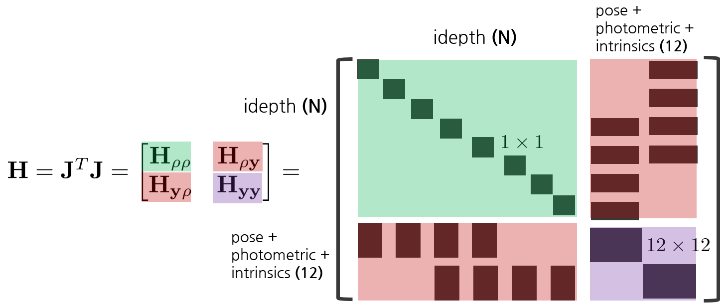
As explained in the Schur Complement section, it takes a lot of time to calculate $\mathbf{H}^{-1}$, so it is calculated in $\Delta \mathbf{x}_{\mathbf{y}}$, $\Delta \mathbf{x}_{\mathbf{\rho}}$ order using Schur Complement.
Details of H and b matrix
The detailed expansion of $\mathbf{H}, \mathbf{b}$ matrices is as follows. This is a good reference when looking at the DSO code and checking which H and b matrix values are being dealt with when matching with the formula.
$$
\begin{bmatrix}
\mathbf{H}_{\rho\rho} & \mathbf{H}_{\rho\mathbf{y}} \\
\mathbf{H}_{\mathbf{y}\rho} & \mathbf{H}_{\mathbf{y}\mathbf{y}}
\end{bmatrix}
=
\begin{bmatrix}
\mathbf{J}_{\rho}^{T}\mathbf{J}_{\rho} & \mathbf{J}_{\rho}^{T}\mathbf{J}_\mathbf{y} \\
\mathbf{J}_{\mathbf{y}}^{T}\mathbf{J}_{\rho} & \mathbf{J}_{\mathbf{y}}^{T}\mathbf{J}_{\mathbf{y}}
\end{bmatrix}
$$
H_yy
$$
\mathbf{H}_{\mathbf{y}\mathbf{y}}
=
\mathbf{J}_{\mathbf{y}}^{T}\mathbf{J}_{\mathbf{y}}
=
\begin{bmatrix}
\mathbf{J}_{\mathbf{c}}^{T}\mathbf{J}_{\mathbf{c}} & \mathbf{J}_{\mathbf{c}}^{T}\mathbf{J}_{\xi'} \\
\mathbf{J}_{\xi'}^{T}\mathbf{J}_{\mathbf{c}} & \mathbf{J}_{\xi'}^{T}\mathbf{J}_{\xi'} \\
\end{bmatrix}
$$
- $\xi' = [ \ \delta \xi \ a \ b \ ]_{8\times1}$
$$
\mathbf{J}_{\mathbf{c}}^{T}\mathbf{J}_{\mathbf{c}}
=
\begin{bmatrix}
\frac{\partial \mathbf{r}^{(1)}}{\partial \mathbf{c}}^{T} & \cdots & \frac{\partial \mathbf{r}^{(N)}}{\partial \mathbf{c}}^{T}
\end{bmatrix}
\begin{bmatrix}
\frac{\partial \mathbf{r}^{(1)}}{\partial \mathbf{c}}
\\
\vdots
\\
\frac{\partial \mathbf{r}^{(N)}}{\partial \mathbf{c}}
\end{bmatrix}
=
\sum^{N}_{i=1}\frac{\partial \mathbf{r}^{(i)}}{\partial \mathbf{c}}^{T}\frac{\partial \mathbf{r}^{(i)}}{\partial \mathbf{c}}
$$
$$
\mathbf{J}_{\mathbf{c}}^{T}\mathbf{J}_{\xi'}
=
\begin{bmatrix}
\frac{\partial \mathbf{r}^{(1)}}{\partial \mathbf{c}}^{T} & \cdots & \frac{\partial \mathbf{r}^{(N)}}{\partial \mathbf{c}}^{T}
\end{bmatrix}
\begin{bmatrix}
\frac{\partial \mathbf{r}^{(1)}}{\partial \xi_{1}} & \cdots & \frac{\partial \mathbf{r}^{(1)}}{\partial \xi_{8}}
\\
\vdots & \ddots & \vdots
\\
\frac{\partial \mathbf{r}^{(N)}}{\partial \xi_{1}} & \cdots & \frac{\partial \mathbf{r}^{(N)}}{\partial \xi_{8}}
\end{bmatrix}
=
\begin{bmatrix}
\sum^{N}_{i=1}\frac{\partial \mathbf{r}^{(i)}}{\partial \mathbf{c}}^{T}\frac{\partial \mathbf{r}^{(i)}}{\partial \xi_{1}} & \cdots & \sum^{N}_{i=1}\frac{\partial \mathbf{r}^{(i)}}{\partial \mathbf{c}}^{T}\frac{\partial \mathbf{r}^{(i)}}{\partial \xi_{8}}
\end{bmatrix}
$$
$$
\mathbf{J}_{\xi'}^{T}\mathbf{J}_{\xi'}
=
\begin{bmatrix}
\frac{\partial \mathbf{r}^{(1)}}{\partial \xi_{1}} & \cdots & \frac{\partial \mathbf{r}^{(1)}}{\partial \xi_{8}}
\\
\vdots & \ddots & \vdots
\\
\frac{\partial \mathbf{r}^{(N)}}{\partial \xi_{1}} & \cdots & \frac{\partial \mathbf{r}^{(N)}}{\partial \xi_{8}}
\end{bmatrix}^{T}
\begin{bmatrix}
\frac{\partial \mathbf{r}^{(1)}}{\partial \xi_{1}} & \cdots & \frac{\partial \mathbf{r}^{(1)}}{\partial \xi_{8}}
\\
\vdots & \ddots & \vdots
\\
\frac{\partial \mathbf{r}^{(N)}}{\partial \xi_{1}} & \cdots & \frac{\partial \mathbf{r}^{(N)}}{\partial \xi_{8}}
\end{bmatrix}
=
\begin{bmatrix}
\sum^{N}_{i=1}\frac{\partial \mathbf{r}^{(i)}}{\partial \xi_{1}}^{T}\frac{\partial \mathbf{r}^{(i)}}{\partial \xi_{1}} & \cdots & \sum^{N}_{i=1}\frac{\partial \mathbf{r}^{(i)}}{\partial \xi_{1}}^{T}\frac{\partial \mathbf{r}^{(i)}}{\partial \xi_{8}}
\\
\vdots & \ddots & \vdots
\\
\sum^{N}_{i=1}\frac{\partial \mathbf{r}^{(i)}}{\partial \xi_{8}}^{T}\frac{\partial \mathbf{r}^{(i)}}{\partial \xi_{1}} & \cdots & \sum^{N}_{i=1}\frac{\partial \mathbf{r}^{(i)}}{\partial \xi_{8}}^{T}\frac{\partial \mathbf{r}^{(i)}}{\partial \xi_{8}}
\end{bmatrix}
$$
H_rho_rho, H_rho_y, H_y_rho
$$
\mathbf{J}_{\rho}^{T}\mathbf{J}_{\rho}
=
\begin{bmatrix}
\frac{\partial \mathbf{r}^{(1)}}{\partial \rho^{(1)}} & \cdots & \frac{\partial \mathbf{r}^{(1)}}{\partial \rho^{(M)}}
\\
\vdots & \ddots & \vdots
\\
\frac{\partial \mathbf{r}^{(N)}}{\partial \rho^{(1)}} & \cdots & \frac{\partial \mathbf{r}^{(N)}}{\partial \rho^{(M)}}
\end{bmatrix}^{T}
\begin{bmatrix}
\frac{\partial \mathbf{r}^{(1)}}{\partial \rho^{(1)}} & \cdots & \frac{\partial \mathbf{r}^{(1)}}{\partial \rho^{(M)}}
\\
\vdots & \ddots & \vdots
\\
\frac{\partial \mathbf{r}^{(N)}}{\partial \rho^{(1)}} & \cdots & \frac{\partial \mathbf{r}^{(N)}}{\partial \rho^{(M)}}
\end{bmatrix}
=
\begin{bmatrix}
\sum^{N}_{i=1}\frac{\partial \mathbf{r}^{(i)}}{\partial \rho^{(1)}}^{T}\frac{\partial \mathbf{r}^{(i)}}{\partial \rho^{(1)}} & 0 & \cdots & 0
\\
0 & \sum^{N}_{i=1}\frac{\partial \mathbf{r}^{(i)}}{\partial \rho^{(2)}}^{T}\frac{\partial \mathbf{r}^{(i)}}{\partial \rho^{(2)}} & \cdots & 0
\\
\vdots & \vdots & \ddots & 0
\\
0 & 0& \cdots & \sum^{N}_{i=1}\frac{\partial \mathbf{r}^{(i)}}{\partial \rho^{(M)}}^{T}\frac{\partial \mathbf{r}^{(i)}}{\partial \rho^{(M)}}
\end{bmatrix}
$$
$$\mathbf{J}_{\mathbf{y}}^{T}\mathbf{J}_{\rho}
=
\begin{bmatrix}
\mathbf{J}_{\mathbf{c}}^{T} & \mathbf{J}_{\xi'}^{T}
\end{bmatrix}^{T}
\mathbf{J}_{\rho}
=
\begin{bmatrix}
\mathbf{J}_{\mathbf{c}}^{T}\mathbf{J}_{\rho} & \mathbf{J}_{\xi'}^{T}\mathbf{J}_{\rho}
\end{bmatrix}^{T}
$$
$$
\mathbf{J}_{\mathbf{c}}^{T}\mathbf{J}_{\rho}
=
\begin{bmatrix}
\frac{\partial \mathbf{r}^{(1)}}{\partial \mathbf{c}}^{T} & \cdots & \frac{\partial \mathbf{r}^{(N)}}{\partial \mathbf{c}}^{T}
\end{bmatrix}
\begin{bmatrix}
\frac{\partial \mathbf{r}^{(1)}}{\partial \rho^{(1)}} & \cdots & \frac{\partial \mathbf{r}^{(1)}}{\partial \rho^{(M)}}
\\
\vdots & \ddots & \vdots
\\
\frac{\partial \mathbf{r}^{(N)}}{\partial \rho^{(1)}} & \cdots & \frac{\partial \mathbf{r}^{(N)}}{\partial \rho^{(M)}}
\end{bmatrix}
=
\begin{bmatrix}
\sum^{N}_{i=1}\frac{\partial \mathbf{r}^{(i)}}{\partial \mathbf{c}}^{T}\frac{\partial \mathbf{r}^{(i)}}{\partial \rho^{(1)}} & \cdots & \sum^{N}_{i=1}\frac{\partial \mathbf{r}^{(i)}}{\partial \mathbf{c}}^{T}\frac{\partial \mathbf{r}^{(i)}}{\partial \rho^{(M)}}
\end{bmatrix}
$$
$$
\mathbf{J}_{\xi'}^{T}\mathbf{J}_{\rho}
=
\begin{bmatrix}
\frac{\partial \mathbf{r}^{(1)}}{\partial \xi_{1}} & \cdots & \frac{\partial \mathbf{r}^{(1)}}{\partial \xi_{8}}
\\
\vdots & \ddots & \vdots
\\
\frac{\partial \mathbf{r}^{(N)}}{\partial \xi_{1}} & \cdots & \frac{\partial \mathbf{r}^{(N)}}{\partial \xi_{8}}
\end{bmatrix}^{T}\begin{bmatrix}
\frac{\partial \mathbf{r}^{(1)}}{\partial \rho^{(1)}} & \cdots & \frac{\partial \mathbf{r}^{(1)}}{\partial \rho^{(M)}}
\\
\vdots & \ddots & \vdots
\\
\frac{\partial \mathbf{r}^{(N)}}{\partial \rho^{(1)}} & \cdots & \frac{\partial \mathbf{r}^{(N)}}{\partial \rho^{(M)}}
\end{bmatrix}
=
\begin{bmatrix}
\sum^{N}_{i=1}\frac{\partial \mathbf{r}^{(i)}}{\partial \xi_{1}}^{T}\frac{\partial \mathbf{r}^{(i)}}{\partial \rho^{(1)}} & \cdots & \sum^{N}_{i=1}\frac{\partial \mathbf{r}^{(i)}}{\partial \xi_{1}}^{T}\frac{\partial \mathbf{r}^{(i)}}{\partial \rho^{(M)}}
\\
\vdots & \ddots & \vdots
\\
\sum^{N}_{i=1}\frac{\partial \mathbf{r}^{(i)}}{\partial \xi_{8}}^{T}\frac{\partial \mathbf{r}^{(i)}}{\partial \rho^{(1)}} & \cdots & \sum^{N}_{i=1}\frac{\partial \mathbf{r}^{(i)}}{\partial \xi_{8}}^{T}\frac{\partial \mathbf{r}^{(i)}}{\partial \rho^{(M)}}
\end{bmatrix}
$$
Since it is $f(\mathbf{x}) = \sqrt{w_{h}}\mathbf{r}$, if the huber norm is omitted and only the residual is expressed, it is as follows.
$$\begin{bmatrix}
\mathbf{b}_{\rho} \\
\mathbf{b}_{\mathbf{y}}
\end{bmatrix}\rightarrow\begin{bmatrix}
\mathbf{J}_{\rho}^{T}f(\mathbf{x}) \\
\mathbf{J}_{\mathbf{y}}^{T}f(\mathbf{x})
\end{bmatrix}\rightarrow\sqrt{w_{h}} \begin{bmatrix}
\mathbf{J}_{\rho}^{T}\mathbf{r} \\
\mathbf{J}_{\mathbf{y}}^{T}\mathbf{r}
\end{bmatrix}$$
In detail, this is as follows.
$$
\mathbf{J}_{\rho}^{T}\mathbf{r}
=
\begin{bmatrix}
\frac{\partial \mathbf{r}^{(1)}}{\partial \rho^{(1)}} & \cdots & \frac{\partial \mathbf{r}^{(1)}}{\partial \rho^{(M)}}
\\
\vdots & \ddots & \vdots
\\
\frac{\partial \mathbf{r}^{(N)}}{\partial \rho^{(1)}} & \cdots & \frac{\partial \mathbf{r}^{(N)}}{\partial \rho^{(M)}}
\end{bmatrix}^{T}
\begin{bmatrix}
\mathbf{r}^{(1)}
\\
\vdots
\\
\mathbf{r}^{(N)}
\end{bmatrix}
=
\begin{bmatrix}
\sum^{N}_{i=1}\frac{\partial \mathbf{r}^{(i)}}{\partial \rho^{(1)}}^{T}\mathbf{r}^{(i)}
\\
\vdots
\\
\sum^{N}_{i=1}\frac{\partial \mathbf{r}^{(i)}}{\partial \rho^{(M)}}^{T}\mathbf{r}^{(i)}
\end{bmatrix}
$$
$$\mathbf{J}_{\mathbf{y}}^{T}\mathbf{r}
=
\begin{bmatrix}
\mathbf{J}_{\mathbf{c}}^{T}
\\
\mathbf{J}_{\xi'}^{T}
\end{bmatrix}
\mathbf{r}
=
\begin{bmatrix}
\frac{\partial \mathbf{r}^{(1)}}{\partial \mathbf{c}}^{T} & \cdots & \frac{\partial \mathbf{r}^{(1)}}{\partial \mathbf{c}}^{T}
\\
\frac{\partial \mathbf{r}^{(1)}}{\partial \xi_{1}}^{T} & \cdots & \frac{\partial \mathbf{r}^{(1)}}{\partial \xi_{8}}^{T}
\\
\vdots & \ddots & \vdots
\\
\frac{\partial \mathbf{r}^{(N)}}{\partial \xi_{1}}^{T} & \cdots & \frac{\partial \mathbf{r}^{(N)}}{\partial \xi_{8}}^{T}
\end{bmatrix}
\begin{bmatrix}
\mathbf{r}^{(1)}
\\
\vdots
\\
\mathbf{r}^{(N)}
\end{bmatrix}
=
\begin{bmatrix}
\sum^{N}_{i=1}\frac{\partial \mathbf{r}^{(i)}}{\partial \mathbf{c}}^{T}\mathbf{r}^{(i)}
\\
\sum^{N}_{i=1}\frac{\partial \mathbf{r}^{(i)}}{\partial \xi_{1}}^{T}\mathbf{r}^{(i)}
\\
\vdots
\\
\sum^{N}_{i=1}\frac{\partial \mathbf{r}^{(i)}}{\partial \xi_{8}}^{T}\mathbf{r}^{(i)}
\end{bmatrix}
$$
4.4. Null Space Effect Elimination
4.4.1. Ambiguity Problems

Since DSO is Visual Odometry using a monocular camera, it has a scale ambiguity problem in which the depth of a map point cannot be accurately determined. For example, it means that it is impossible to know exactly whether I am currently looking at an image of a real city or a miniature image of a city using only a monocular camera. In other words, even if the trajectory of the camera and all map points are collectively increased or decreased, it has no effect in the optimization stage.

Also, if the same SE(3) transform is applied to all camera poses and map points, this also has no effect in the optimization step. This is called the coordinate system ambiguity problem. (For more info see(https://blog.csdn.net/wubaobao1993/article/details/105106301)
4.4.2. Null Space
When a square matrix $\mathbf{A} \in \mathbb{R}^{n\times n}$ and a vector $\mathbf{x} \in \mathbb{R}^{n}$ exist, the following means a solution set that satisfies.
$$\mathbf{Ax} = 0$$
In general, when using the Gauss-Newton (GN) method, a situation arises in which the following formula must be solved.
$$\mathbf{H}\Delta \mathbf{x} = -\mathbf{b}$$
- $\mathbf{H} = \mathbf{J}^{T}\mathbf{J} \in \mathbb{R}^{n\times n}$
- $\mathbf{b} = \mathbf{J}^{T}\mathbf{e}\in \mathbb{R}^{n}$
- $\Delta \mathbf{x} \in \mathbb{R}^{n}$
If the inverse of $\mathbf{H}$ exists, then $\Delta \mathbf{x}$ has a unique solution
$$\Delta \mathbf{x} = -\mathbf{H}^{-1}\mathbf{b} \quad \text{if } \mathbf{H} \text{ is invertible}$$
If the inverse of $\mathbf{H}$ does not exist, $\Delta \mathbf{x}$ has a special solution and is a homogeneous solution with $\Delta \mathbf{x}_{p}$ It has a complete solution by adding $\Delta \mathbf{x}_{h}$.
$$\Delta \mathbf{x} = \Delta \mathbf{x}_{h} + \Delta \mathbf{x}_{p} \quad \text{if } \mathbf{H} \text{ is not invertible}$$
First of all, the special solution $\Delta \mathbf{x}_{p}$ can be obtained from a non-homogeneous equation.
$$\mathbf{H}\Delta \mathbf{x}_{p} = -\mathbf{b}$$
Next, the general solution $\Delta \mathbf{x}_{h}$ can be obtained from the homogeneous equation.
$$\mathbf{H}\Delta \mathbf{x}_{h} = 0$$
Therefore, if the inverse of $\mathbf{H}$ does not exist, the complete solution can be expressed as follows. At this time, $\lambda$ means an arbitrary integer, and since the equation below always holds regardless of the value of $\lambda$, the complete solution has infinitely many solutions.
$$\Delta \mathbf{x} = \Delta \mathbf{x}_{p} + \lambda \Delta \mathbf{x}_{h} $$
$$\mathbf{H}(\Delta \mathbf{x}_{p} + \lambda \Delta \mathbf{x}_{h}) = -\mathbf{b} $$
Here, the null space means the space spanned by the solution set of $\Delta \mathbf{x}_{h}$.
$$\mathbf{N} = \text{Span}(\Delta \mathbf{x}_{h}) $$
Since the null space does not affect the value of the entire equation, $\mathbf{N}\Delta \mathbf{x}$, a linear combination of null spaces, is also included in the null space, resulting in the following equation.
More about this source text
$$\mathbf{H}\Delta \mathbf{x} + \mathbf{N}\Delta \mathbf{x}= -\mathbf{b} $$
4.4.3. Null Space in DSO

The null space does not affect the system(= error function) $\|\mathbf{E}(\mathbf{x} + \Delta \mathbf{x})\|$ value, but does affect the update value $\Delta \mathbf{x}$, so the effect of the null space is the cause of the ambiguity problem. Therefore, DSO used a method to solve the ambiguity problem by removing the effect of the null space when performing LBA.

For example, assuming that the update value $\Delta \mathbf{x} = \Delta \mathbf{x}_{p} + \Delta \mathbf{x}_{h} $ is obtained through LBA as shown in the figure above. Here, the effect of the null space can be removed by subtracting the amount $\mathbf{P}_{N}\Delta \mathbf{x}$ projected into the null space.
The projection matrix $\mathbf{P}_{N}$ can be obtained in two ways depending on whether an inverse matrix of $\mathbf{N}^{T}\mathbf{N}$ exists or not.
\begin{equation*}
\begin{aligned}
\mathbf{P}_{\mathbf{N}} & = \mathbf{NN}^{\dagger} \\
& = \mathbf{N}(\mathbf{N}^{T}\mathbf{N})^{-1}\mathbf{N}^{T} \quad \text{if, } \mathbf{NN}^{T} \ \text{is invertible.} \\
& = \mathbf{N}(\mathbf{V}\Sigma^{\dagger}\mathbf{U}^{T}) \quad \text{if, } \mathbf{NN}^{T} \ \text{is not invertible. Do SVD}
\end{aligned}
\end{equation*}
In conclusion, the effect of the null space can be removed by calculating the optimal update value $\Delta \mathbf{x}^{*} $ as follows.
$$\Delta \mathbf{x}^{*} = \Delta \mathbf{x} - \mathbf{NN}^{\dagger} \Delta \mathbf{x}$$
4.4.4. Detailed Derivation of Null Space in DSO
Deriving by another method without using a projection matrix is as follows. First of all, the optimal update value $\Delta \mathbf{x}^{*} $ can be expressed as follows. At this time, $\mathbf{N}\Delta \mathbf{x}_{h}$ means the value drifted by the null space.
$$\Delta \mathbf{x}^{*} = \Delta \mathbf{x} - \mathbf{N}\Delta \mathbf{x}_{h}$$
Using the fact that the null space does not affect the value of the error function, the following formula holds.
\begin{equation*}
\begin{aligned}
\mathbf{E}(\mathbf{x}+\Delta \mathbf{x}) = \mathbf{E}(\mathbf{x} + \Delta \mathbf{x} - \mathbf{N}\Delta \mathbf{x}_{h})
\end{aligned}
\end{equation*}
If the two error functions in the above formula are rearranged by first-order Taylor expansion, it can be expressed as follows.
\begin{equation*}
\begin{aligned}
\mathbf{E}(\mathbf{x} + \Delta\mathbf{x} - \mathbf{N}\Delta \mathbf{x}_{h}) & = \mathbf{e}(\mathbf{x}+\Delta \mathbf{x} - \mathbf{N}\Delta \mathbf{x}_{h})^{T}\mathbf{e}(\mathbf{x}+\Delta \mathbf{x} - \mathbf{N}\Delta \mathbf{x}_{h}) \\
& \simeq (\mathbf{e}(\mathbf{x}) + \mathbf{J}(\Delta \mathbf{x}-\mathbf{N}\Delta \mathbf{x}_{h}))^{T}(\mathbf{e}(\mathbf{x}) + \mathbf{J}(\Delta \mathbf{x}-\mathbf{N}\Delta \mathbf{x}_{h})) \\
& = \underbrace{\mathbf{e}^{T}\mathbf{e} + \mathbf{e}^{T}\mathbf{J}\Delta \mathbf{x} + \Delta \mathbf{x}\mathbf{J}^{T}\mathbf{e} + \Delta \mathbf{x}^{T}\mathbf{J}^{T}\mathbf{J}\Delta \mathbf{x}}_{\mathbf{E}(\mathbf{x}+\Delta \mathbf{x})}
\underbrace{-\mathbf{e}^{T}\mathbf{JN}\Delta \mathbf{x}_{h} - (\mathbf{N}\Delta \mathbf{x}_{h})^{T}\mathbf{J}^{T}\mathbf{e} - (\mathbf{N}\Delta \mathbf{x}_{h})^{T}\mathbf{J}^{T}\mathbf{J}\Delta \mathbf{x} - \Delta \mathbf{x} \mathbf{J}^{T}\mathbf{J}(\mathbf{N}\Delta \mathbf{x}_{h}) + (\mathbf{N}\Delta \mathbf{x}_{h})^{T}\mathbf{J}^{T}\mathbf{J}(\mathbf{N}\Delta \mathbf{x}_{h})}_{\Delta \mathbf{x}_{h} \ part} \\
& = \mathbf{E}(\mathbf{x} + \Delta \mathbf{x})
\end{aligned}
\end{equation*}
Therefore, after eliminating the common part, rearranging again, the following formula is established.
\begin{equation*}
\begin{aligned}
(\mathbf{N}\Delta \mathbf{x}_{h})^{T}\mathbf{J}^{T}\mathbf{J}(\mathbf{N}\Delta \mathbf{x}_{h}) = \mathbf{e}^{T}\mathbf{JN}\Delta \mathbf{x}_{h} + (\mathbf{N}\Delta \mathbf{x}_{h})^{T}\mathbf{J}^{T}\mathbf{e} + (\mathbf{N}\Delta \mathbf{x}_{h})^{T}\mathbf{J}^{T}\mathbf{J}\Delta \mathbf{x} + \Delta \mathbf{x} \mathbf{J}^{T}\mathbf{J}(\mathbf{N}\Delta \mathbf{x}_{h})
\end{aligned}
\end{equation*}
Here, $\mathbf{N}\Delta \mathbf{x}_{h}$ corresponding to the linear combination of the null space and $\mathbf{J}^{T}\mathbf{e}$ representing the gradient of the error function are orthogonal to each other, so the following holds.
$$\mathbf{N}\Delta \mathbf{x}_{h}\mathbf{J}^{T}\mathbf{e} = 0$$
So, rearranging the remaining equations, we obtain the following equation:
$$\mathbf{N}\Delta \mathbf{x}_{h} = \Delta \mathbf{x}$$
However, since the above formulas do not actually match each other, if an approximate solution is obtained using least squares for $\Delta \mathbf{x}_{h}$, an approximate solution that minimizes the magnitude of $\| \mathbf{N}\Delta \mathbf{x}_{h} - \Delta \mathbf{x}\|$ can be obtained. At this time, depending on whether the inverse matrix of $\mathbf{N}^{T}\mathbf{N}$ exists or not, the solution can be obtained as follows.
\begin{equation*}
\begin{aligned}
& \Delta \mathbf{x}_{h} = \mathbf{N}^{\dagger}\Delta \mathbf{x} \quad \text{if, } \mathbf{NN}^{T} \ \text{ is invertible.} \\
& \Delta \mathbf{x}_{h} = \mathbf{V}\mathbf{D}^{\dagger}\mathbf{U}^{T}\Delta \mathbf{x} \quad \text{if, } \mathbf{NN}^{T} \ \text{ is not invertible.} \\
\end{aligned}
\end{equation*}
In conclusion, we can calculate the optimal update value $\Delta \mathbf{x}^{*} $ as follows.
$$\Delta \mathbf{x}^{*} = \Delta \mathbf{x} - \mathbf{N}\Delta \mathbf{x}_{h} \Rightarrow \Delta \mathbf{x}^{*} = \Delta \mathbf{x} - \mathbf{NN}^{\dagger} \Delta \mathbf{x}$$
$\mathbf{H}^{*}, \mathbf{b}^{*}$ with null space effect removed can be derived as follows.
\begin{equation*}
\begin{aligned}
\Delta \mathbf{x}^{T} \mathbf{b}^{*} & = \Delta \mathbf{x}^{T} \mathbf{b} - \Delta \mathbf{x}_{h}^{T}\mathbf{b}_{n} \\
& = \Delta \mathbf{x}^{T} \mathbf{b} - (\mathbf{N}^{\dagger}\Delta \mathbf{x})^{T}\mathbf{N}^{T}\mathbf{J}^{T}\mathbf{e} \\
& = \Delta \mathbf{x}^{T}\mathbf{b} - \Delta \mathbf{x}^{T}(\mathbf{NN}^{\dagger})^{T}\mathbf{b} \\
& = \text{where, } \mathbf{b}_{n} = \mathbf{J}_{n}\mathbf{e} \ \ \mathbf{J}_{n} = \frac{\partial \mathbf{e}}{\partial \Delta \mathbf{x}_{h}} = \frac{\partial \mathbf{e}}{\partial \Delta \mathbf{x}}\frac{\partial \Delta \mathbf{x}}{\partial \Delta \mathbf{x}_{h}} = \mathbf{JN}
\end{aligned}
\end{equation*}
\begin{equation*}
\begin{aligned}
\Delta \mathbf{x}^{T} \mathbf{H}^{*} \Delta \mathbf{x} & = \Delta \mathbf{x}^{T} \mathbf{H}\Delta \mathbf{x} - \Delta \mathbf{x}_{h}^{T}\mathbf{H}_{n}\Delta \mathbf{x}_{h} \\
& = \Delta \mathbf{x}^{T}\mathbf{H}\Delta \mathbf{x} - (\mathbf{N}^{\dagger}\Delta \mathbf{x})^{T}\mathbf{N}^{T}\mathbf{J}^{T}\mathbf{JN}(\mathbf{N}^{\dagger}\Delta \mathbf{x}) \\
& = \Delta \mathbf{x}^{T} \mathbf{H} \Delta \mathbf{x} - \Delta \mathbf{x}^{T}(\mathbf{NN}^{\dagger})^{T} \mathbf{H} (\mathbf{NN}^{\dagger})\Delta \mathbf{x} \\
& \text{where, } \mathbf{H}_{n} = \mathbf{J}_{n}^{T}\mathbf{J}_{n}, \ \ \mathbf{J}_{n} = \frac{\partial \mathbf{e}}{\partial \Delta \mathbf{x}_{h}} = \frac{\partial \mathbf{e}}{\partial \Delta \mathbf{x}}\frac{\partial \Delta \mathbf{x}}{\partial \Delta \mathbf{x}_{h}} = \mathbf{JN}.
\end{aligned}
\end{equation*}
Therefore, the effect of the null space can be finally removed through the following operation.
$$\mathbf{b}^{*} = \mathbf{b} - (\mathbf{NN}^{\dagger})^{T}\mathbf{b}$$
$$\mathbf{H}^{*} = \mathbf{H} - (\mathbf{NN}^{\dagger})^{T}\mathbf{H}(\mathbf{NN}^{\dagger})$$
5. Pixel Selection
5.1. Make Histogram
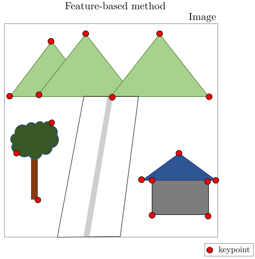
In the case of feature-based VOs such as ORB-SLAM2, keypoints are extracted using a feature extraction algorithm when a specific point is extracted from an image. Then, unprojection $\pi^{-1}(\cdot)$ of the corresponding keypoint into a 3D point and reprojection $\pi(\cdot)$ into a 2D point again to calculate the motion of the camera using the reprojection error. .

However, since the DSO using the direct method calculates the brightness error of a specific pixel without the process of extracting the keypoint, the method of extracting the specific point is also different from the feature-based method. In DSO, gradient histogram and dynamic grid methods were used to extract specific points from images.
The method is not 100% accurate because the DSO paper lacks a detailed explanation, there are no reference papers, and there is little information even when googled. It would be nice to see the contents as a reference when reading the thesis.
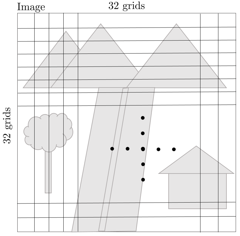
1. First of all, when a new image comes in, the image is divided into 32x32 areas to create a gradient histogram. (grayscale)
2. When one area is enlarged, the picture below is composed of several pixels, and each pixel has its own brightness value. Using this, you can obtain an image gradient (dx,dy) and create a histogram for that area.

3. At this time, the gradient $dx,dy$ originally has a value of 0 to 255, but in DSO, a histogram is created using the value of bin = $\sqrt{dx^{2}+dy^{2}}$ of one pixel. Created.
$$0<\sqrt{dx^{2}+dy^{2}}<360$$
The bin has the same range as above, but it is limited to the range of 1 to 50, and the range of the histogram is simplified by setting the maximum value to 50 if it exceeds 50.

4. Compute this histogram over all 32x32 areas.


5. Find bin values that are 50% of the total count in the histogram in order of 1-50. For example, if a total of 1000 items are counted in all bins of the histogram, count values are sequentially subtracted from bin 1, and the bin whose corresponding value is less than 500 is set as the threshold. In addition, a smoothed threshold value using the threshold average of the surrounding 3x3 area is also set.
5.2. Dynamic Grid

After creating a 32x32 histogram for an image and setting a threshold value, pixels are selected within the image through the dynamic grid method. Through this, it is possible to prevent most of the points from being extracted in the high gradient area and to manage the total number of points (N=2000) that can be extracted from one image.
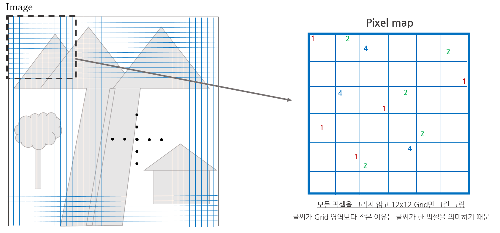
1. Set the size of one grid area. DSO used 12x12 [pixel] as the initial value. Based on a 640x480 image, a size smaller than the 32x32 histogram area is generally used. If the grid size is set, the entire image is divided into grids.
2. Zooming in on one grid area is shown below. At this time, the gradient of a total of three pyramid images is used in one area. Referring to Alalagong's data, if each pyramid is marked with blue (lv2), green (lv1), and red (lv0, original), the pixels in the corresponding area are searched in order as shown in the figure below.

3. From the place where the pyramid level is low (lv0, original), the smoothed threshold value of the histogram of the corresponding area is compared with the squared gradient $\sqrt{dx^{2}+dy^{2}}$ value of the pixel while looping one pixel at a time. (111 -> 112 -> 113 -> ... -> 119 -> 11 -> 1 -> 121 -> 122 -> 123 -> ... -> 129 -> 12 -> 2 -> ...)
At this time, if the specific pixel value is greater than the smoothed threshold, the next step is to calculate the $(dx,dy)$ value of the pixel and the random direction vectors, randdir and norm, and check whether the corresponding value is greater than 0.
$$\text{randdir} \cdot (dx,dy) > 0$$
4. Finally, if norm is greater than a specific value, the corresponding pixel is selected as the pixel representing the grid and the loop is escaped.
ex) If the $\sqrt{dx^{2}+dy^{2}}$ value of 115 pixels is greater than the smoothed threshold and satisfies $\text{randdir} \cdot (dx_{115},dy_{115}) > 0$, 115 pixels are selected as grid representative pixels and the loop is escaped. By calculating a random direction vector and norm, we prevented point extraction from concentrating on a specific pixel area.
5. If the pixel is smaller than the smoothed threshold, the values are compared in the order of lv0 -> lv1 -> lv2. At this time, the higher the level, the threshold is multiplied by 0.75, and then compared with the pixel brightness value, the higher the pyramid level, the higher the probability of being extracted.
6. If the total number of extracted points is less than the desired total amount (default N=2000) even though all pixels have been inspected ($N_{\text{want}}/N_{\text{have}} > 1.25 $), the Search again after reducing the size of one grid, and if there are too many extracted points ($N_{\text{want}}/N_{\text{have}} < 0.25$), the points are extracted again with a 16x16 grid size. .

7. Loop through all grids within an image and store only pixels that pass the smoothed threshold in the pixel map. In the pixel map, a point extracted from lv0 has a value of '1', a point extracted from lv1 has a value of '2', and a point extracted from lv3 has a value of '4'. The value of the area where no points are extracted has '0'.
6. Code Review
References
1. [EN] DSO paper
2. [KR] SLAMKR study
3. [CH] DSO code reading
4. [CH] jingeTU's SLAM blog
5. [CH] DSO tracking and optimization
6. [CH] DSO initialization
7. [CH] Detailed in DSO
8. [CH] DSO photometric calibration
9. [CH] DSO code with comments
10.[CH] DSO Null Space
11. [CH] DSO (5) Calculation and Derivation of Null Space
12. [KR] goodgodgd's Visual Odometry and vSLAM
13.[EN] DSO Photometric Calibration paper
'English' 카테고리의 다른 글
| [En] Notes on Multiple View Geometry in Computer Vision Part 1 (0) | 2023.01.18 |
|---|---|
| [SLAM][En] Direct Sparse Odometry (DSO) Paper Review Part 1 (0) | 2023.01.17 |
| [En] Notes on Lie Theory (SO(3), SE(3)) (0) | 2023.01.17 |
| [En] Notes on Plücker Coordinate (0) | 2023.01.17 |
| [SLAM][En] Errors and Jacobian Derivations for SLAM Part 2 (0) | 2023.01.17 |
 A L I D A


