 A L I D A
Youtube
다중관점기하학(Multiple View Geometry) 개념 정리
www.youtube.com
0. Projective Space
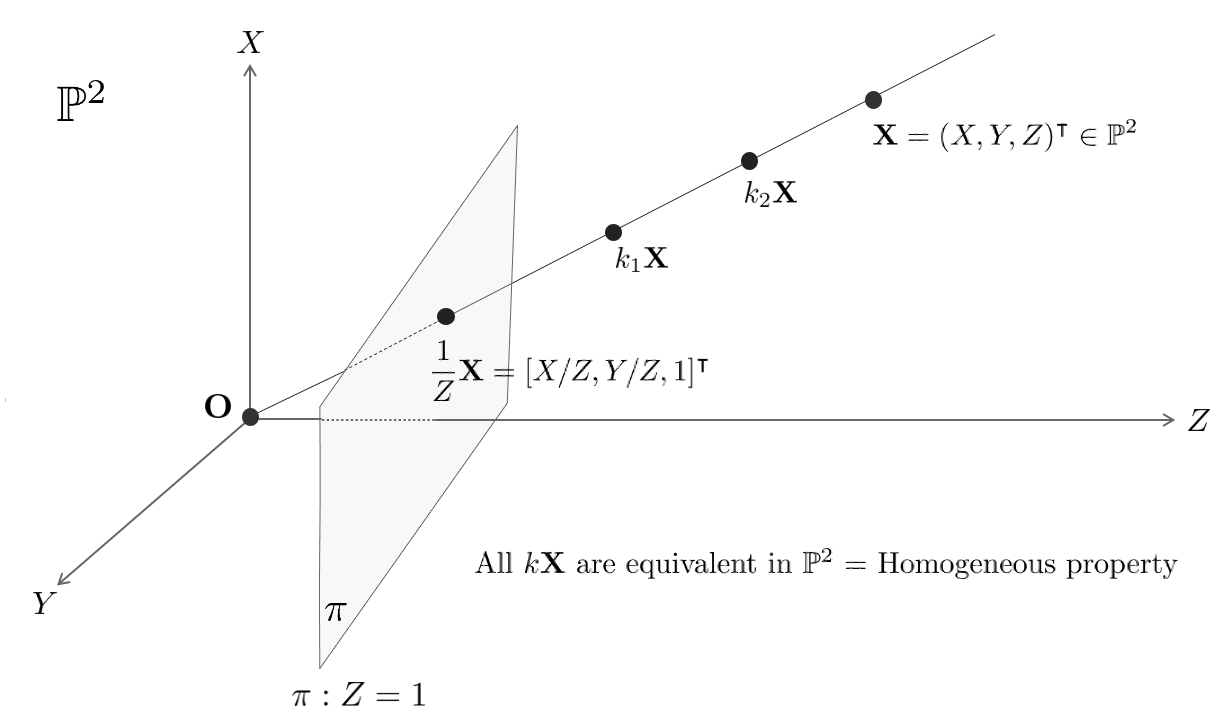
사영 공간(projective space) $\mathbb{P}^{n}$는 $\mathbb{R}^{n+1}$ 공간 상의 원점을 지나는 직선들의 집합을 의미한다. 따라서 원점을 제외한 $\mathbb{R}^{n+1}$ 공간 상의 모든 원소를 포함한다. 엄밀히 말하면 허수를 제외한 실수만 취급하므로 $\mathbb{RP}^{n}$라고 써야하지만 본 포스팅에서는 편의를 위해 $\mathbb{P}^{n}$를 사용한다.
\begin{equation}
\begin{aligned}
\mathbb{P}^{n} = \mathbb{R}^{n+1} - \{0\} \\
\end{aligned}
\end{equation}
3차원 공간 상에 점 $\mathbf{X}$가 다음과 같이 주어졌다고 하자.
\begin{equation}
\begin{aligned}
& \mathbf{X} = [X, Y, Z]^{\intercal} \\
\end{aligned}
\end{equation}
$\mathbf{X}$의 모든 원소에 임의의 값 $k$를 곱해도 이는 원점과 $\mathbf{X}$를 잇는 직선 위에 존재하며 이러한 성질을 homogeneous 성질이라고 한다. 만약 $k=1/Z$를 곱해주면 3차원 점을 $Z=1$ 평면에 프로젝션한 것과 기하학적으로 동일한 의미를 지닌다.
\begin{equation}
\begin{aligned}
& [X, Y, Z]^{\intercal} \rightarrow [X/Z, Y/Z, 1]^{\intercal}
\end{aligned}
\end{equation}
따라서 $\mathbb{P}^{2}$을 사용하면 3차원 공간 상의 점들을 특정 평면에 프로젝션하여 $\mathbb{R}^{2}$와 동일하게 2차원 공간 상의 점, 직선, 곡면 등을 표현할 수 있고 여기에 추가적으로 무한대 점(point at infinity) $\mathbf{x}_{\infty}$과 무한대 직선(line at infinity) $\mathbf{l}_{\infty}$를 표현할 수 있는 표현의 이점을 지닌다. 또한 점과 직선을 동일한 3차원 벡터로 연산할 수 있는 연산의 이점을 지닌다. 자세한 내용은 추후 섹션에서 설명한다.
1. Projective geometry and transformations in 2D
1.1. The 2D projective plane
일반적으로 평면 위의 점 $\mathbf{x}$는 $(x,y) \in \mathbb{R}^{2}$와 같이 표현한다. $\mathbb{R}^{2}$가 벡터공간(vector space)이라고 하면 $\mathbf{x}$는 하나의 벡터로 나타낼 수 있다. 또한, 두 점 $\mathbf{x}_{1}, \mathbf{x}_{2}$을 포함하는 직선 $\mathbf{l}$은 두 벡터를 뺌으로써 표현할 수 있다. 해당 섹션에서는 평면 위의 점과 직선에 대해 하나의 동일한 벡터로 표현할 수 있게 해주는 homogeneous notation에 대해 설명한다.
1.1.1. Points and lines
1.1.2. Homogeneous representation of line
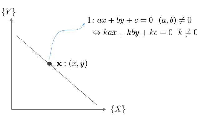
임의의 직선 $\mathbf{l}$은 다음과 같이 표현할 수 있다.
\begin{equation}
\begin{aligned}
\mathbf{l}: ax + by + c = 0 \quad (a,b) \neq 0
\end{aligned}
\end{equation}
직선 $\mathbf{l}$ 위에 임의의 한 점 $\mathbf{x} = (x,y,1)$이 존재하면 직선 $ax+by+c=0$ 공식에 따라 직선 $\mathbf{l}$은 다음과 같이 표현할 수 있다.
\begin{equation}
\begin{aligned}
& \mathbf{l} : (a,b,c) \\
\end{aligned}
\end{equation}
이 때, $(a,b,c)$는 직선 $\mathbf{l}$을 유일하게 표현하지 않는다. $(ka,kb,kc)$와 같이 0이 아닌 임의의 상수 $k$를 곱해도 동일한 직선 $\mathbf{l}$을 표현할 수 있다.
\begin{equation}
\begin{aligned}
\mathbf{l}: (ka,kb,kc)
\end{aligned}
\end{equation}
따라서 평면 위의 직선 $\mathbf{l}$은 스케일 값에 상관없이 모두 같은 직선을 의미 한다. 이러한 동치관계(equivalent)에 있는 모든 벡터를 homogeneous 벡터라고 한다. $\mathbb{R}^{3}$ 공간에서 동치관계에 있는 모든 벡터들의 집합을 사영공간(projective space) $\mathbb{P}^{2}$이라고 한다.
1.1.3. Homogeneous representation of points
직선 $\mathbf{l}=(a,b,c)^{\intercal}$과 직선 위의 한 점 $\mathbf{x}=(x,y)^{\intercal}$ 사이에는 다음 공식이 성립한다.
\begin{equation}
\begin{aligned}
ax+by+c=0
\end{aligned}
\end{equation}
이는 두 벡터 $\mathbf{l}$과 $\mathbf{x}$의 내적으로 표현할 수 있다.
\begin{equation}
\begin{aligned}
\begin{pmatrix} x&y&1 \end{pmatrix} \begin{pmatrix} a\\b\\c \end{pmatrix} = \begin{pmatrix} x&y&1 \end{pmatrix}\mathbf{l} = 0
\end{aligned}
\end{equation}
이는 직선 위의 한 점 $\mathbf{x}=(x,y)$ 좌표 맨 끝에 1을 추가하여 직선과 내적한 것으로 볼 수 있다. 직선 $\mathbf{l}$는 스케일 값에 상관없이 하나의 직선을 표현할 수 있으므로 $(x,y,1)\mathbf{l}=0$이 성립한다는 전제하에 모든 $k$값에 대해 $(kx,ky,k)\mathbf{l}=0$ 또한 성립한다. 따라서 임의의 상수 $k$에 대해서 $(kx,ky,k)$는 $\mathbb{R}^{2}$ 공간에서 한 점 $\mathbf{x}=(x,y)$를 의미하므로 직선과 동일하게 점 또한 homogeneous 벡터로 표현할 수 있다. 이를 일반화하여 표현하면 임의의 점 $\mathbf{x}=(x,y,z)^{\intercal}$는 $\mathbb{R}^{2}$ 공간 상의 한 점 $(x/z,y/z)$을 표현한다.
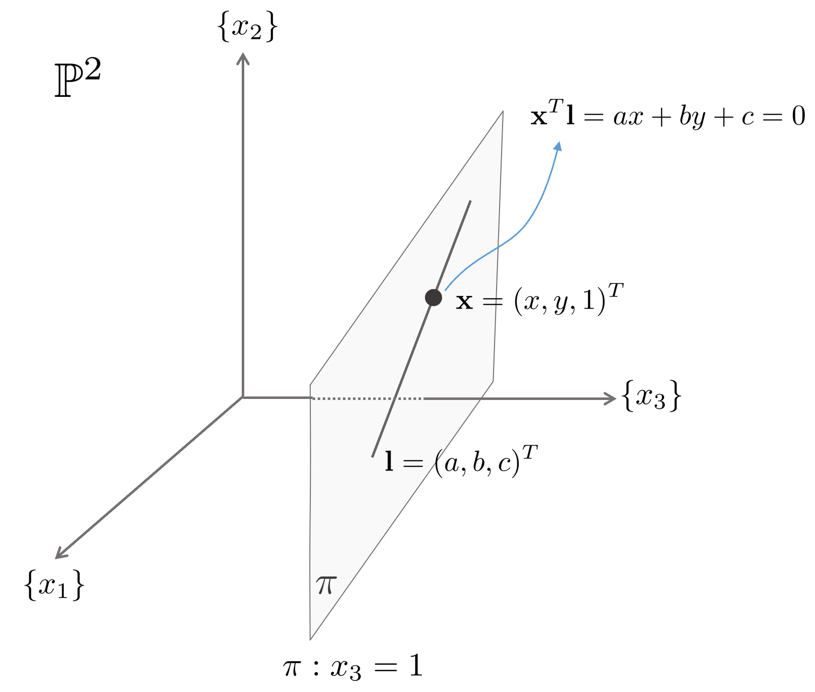
따라서 $\mathbb{P}^{2}$ 공간 상에서 임의의 한 점 $\mathbf{x}$가 직선 $\mathbf{l}$ 위에 존재할 경우
\begin{equation}
\begin{aligned}
\mathbf{x}^{\intercal}\mathbf{l} & = \begin{bmatrix} x&y&1 \end{bmatrix} \begin{bmatrix} a\\b\\c \end{bmatrix} \\
& = ax + by + c \\
& = 0 \\
& \therefore \mathbf{x}^{\intercal}\mathbf{l} = 0
\end{aligned}
\end{equation}
공식이 성립한다.
1.1.4. Degree of freedom (dof)
$\mathbb{P}^{2}$ 공간에서 하나의 점이 유일하게 결정되기 위해서는 반드시 2개의 값 $(x,y)$가 주어져야 한다. 직선을 유일하게 결정하기 위해서는 두 개의 독립적인 $\{a:b:c\}$ 비율이 주어져야 한다. 이와 같이 $\mathbb{P}^{2}$ 공간에서 점과 직선은 2자유도를 가진다.
1.1.5. Intersection of lines
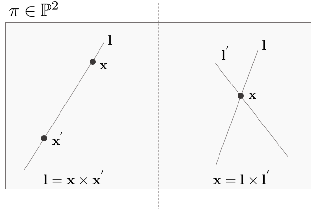
$\mathbb{P}^{2}$ 공간 상의 두 개의 직선 $\mathbf{l}, \mathbf{l}^{\prime}$이 주어졌을 때 두 직선의 방정식은 다음과 같이 쓸 수 있다.
\begin{equation}
\begin{aligned}
& \mathbf{x}^{\intercal}\mathbf{l} = 0 \\
& \mathbf{x}^{\intercal}\mathbf{l}^{\prime} = 0 \\
\end{aligned}
\end{equation}
이 때, 교차점 $\mathbf{x}$는 스케일 값에 관계없이 하나의 점을 의미하므로 두 직선 $\mathbf{l}, \mathbf{l}^{\prime}$의 cross product의 배수로 나타낼 수 있다.
\begin{equation}
\begin{aligned}
\mathbf{x} = \mathbf{l} \times \mathbf{l}^{\prime}
\end{aligned}
\end{equation}
예를 들어, $\mathbb{P}^{2}$ 공간에 $x=1$인 직선과 $y=1$인 직선이 존재하면 두 직선은 $(1,1)$에서 교점을 가진다. 이를 위 공식을 이용해서 구해보면 직선 $x=1$은 $-x+1=0 \Rightarrow (-1,0,1)^{\intercal}$로 표현할 수 있고 직선 $y=1$은 $-y+1=0 \Rightarrow (0,-1,1)^{\intercal}$로 표현할 수 있으므로
\begin{equation}
\begin{aligned}
\mathbf{x} = \mathbf{l}\times \mathbf{l}^{\prime} = \begin{vmatrix} \mathbf{I}&\mathbf{j}&\mathbf{k} \\ -1&0&1 \\ 0&-1&1 \end{vmatrix} = \begin{pmatrix} 1\\1\\1 \end{pmatrix}
\end{aligned}
\end{equation}
가 성립한다. $(1,1,1)^{\intercal}$는 $\mathbb{R}^{2}$ 공간에서 $(1,1)$을 의미한다.
1.1.6. Line joining points
두 직선의 교점을 구하는 공식과 유사하게 $\mathbb{P}^{2}$ 공간에서 두 점 $\mathbf{x}, \mathbf{x}^{\prime}$가 주어졌을 때 두 점을 지나는 직선 $\mathbf{l}$은 다음과 같이 구할 수 있다.
\begin{equation}
\begin{aligned}
\mathbf{l} = \mathbf{x} \times \mathbf{x}^{\prime}
\end{aligned}
\end{equation}
1.2. Ideal points and the line at infinity
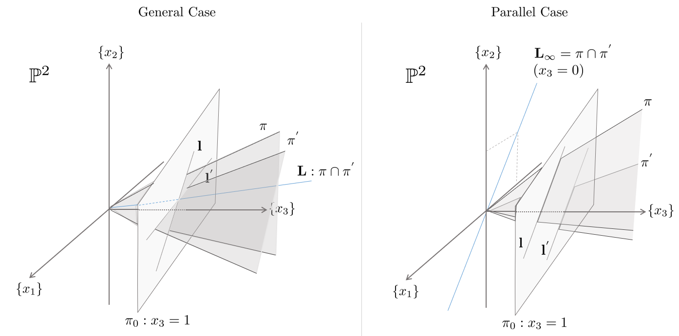
1.2.1. Intersection of parallel lines
만약 두 직선 $\mathbf{l}, \mathbf{l}^{\prime}$이 평행한 경우 두 직선의 교차점은 $\mathbb{R}^{2}$ 공간에서는 만나지 않지만 $\mathbb{P}^{2}$ 공간에서는 만난다.
\begin{equation}
\begin{aligned}
\mathbb{P}^{2} = \mathbb{R}^{2} \cup \mathbf{l}_{\infty}
\end{aligned}
\end{equation}
평행한 두 직선 $\mathbf{l}, \mathbf{l}^{\prime}$은 다음과 같이 나타낼 수 있다.
\begin{equation}
\begin{aligned}
& \mathbf{l}: (a,b,c)^{\intercal} \\
& \mathbf{l}^{\prime}: (a,b,c^{\prime})^{\intercal} \\
\end{aligned}
\end{equation}
평행한 두 직선은 무한대에 위치한 점 $\mathbf{x}_{\infty}$에서 교차하므로
\begin{equation}
\begin{aligned}
\mathbf{x}_{\infty} & = \mathbf{l} \times \mathbf{l}^{\prime} \\
& = (c^{\prime}-c)\begin{pmatrix} b \\ -a \\ 0 \end{pmatrix} \sim \begin{pmatrix} b \\ -a \\ 0 \end{pmatrix}
\end{aligned}
\end{equation}
공식이 성립한다. 이러한 무한대 점 $\mathbf{x}_{\infty}$를 $\mathbb{R}^{2}$ 공간으로 변환하면 $(b/0,-a/0)$이 되어 유효하지 않는 점으로 변환된다. 따라서 $\mathbb{P}^{2}$ 공간에서 무한대 점 $\mathbf{x}_{\infty}=(x,y,0)^{\intercal}$는 $\mathbb{R}^{2}$ 공간으로 변환되지 않는다. 이를 통해 euclidean 공간에서 평행한 두 직선은 만나지 않지만 사영 공간(projective space)에서는 무한대에서 만난다는 것을 알 수 있다.
예를 들어 $\mathbb{P}^{2}$ 공간에 평행한 두 직선 $x=1$과 $x=2$가 주어지면 두 직선은 무한대에서 교차한다. 이를 homogeneous notation으로 표현하면 $-x+1=0 \Rightarrow (-1,0,1)^{\intercal}$ 그리고 $-x+2=0 \Rightarrow(-1,0,2)^{\intercal}$이므로
\begin{equation}
\begin{aligned}
\mathbf{x}_{\infty} = \mathbf{l} \times \mathbf{l}^{\prime} = \begin{vmatrix} \mathbf{I}&\mathbf{j}&\mathbf{k} \\ -1&0&1 \\ -1&0&2 \end{vmatrix} = \begin{pmatrix} 0\\1\\0 \end{pmatrix}
\end{aligned}
\end{equation}
이 된다. 이 때, $\mathbf{x}_{\infty}$는 y축 방향의 무한대 점을 의미한다.
1.2.2. Ideal points and the line at infinity
homogeneous 벡터 $\mathbf{x}=(x_{1},x_{2},x_{3})^{\intercal}$는 $x_{3} \neq 0$일 때 $\mathbb{R}^{2}$ 공간 상의 한 점과 대응된다. 그러나 $x_{3} =0$이면 해당 점은 $\mathbb{R}^{2}$ 공간과 대응되지 않고 $\mathbb{P}^{2}$ 공간에만 존재하는데 이를 ideal point 또는 무한대 점(point at infinity)라고 부른다. 무한대 점은
\begin{equation}
\begin{aligned}
\mathbf{x}_{\infty} = \begin{pmatrix} x_{1}&x_{2}&0 \end{pmatrix}^{\intercal}
\end{aligned}
\end{equation}
와 같은 형태를 갖는다. 이러한 무한대 점들은 특정한 직선 위에 존재하게 되는데 이러한 직선을 무한대 직선(line at infinity)라고 한다.
\begin{equation}
\begin{aligned}
\mathbf{l}_{\infty} = \begin{pmatrix} 0&0&1 \end{pmatrix}^{\intercal}
\end{aligned}
\end{equation}
따라서 $\mathbf{x}_{\infty}^{\intercal}\mathbf{l}_{\infty} = \begin{pmatrix} x_{1}&x_{2}&0 \end{pmatrix}\begin{pmatrix} 0&0&1 \end{pmatrix}^{\intercal} = 0$이 성립한다.
이전 섹션에서 설명한 것과 같이 두 평행한 직선 $\mathbf{l}=(a,b,c)^{\intercal}$과 $\mathbf{l}_{\infty}^{\prime}=(a,b,c^{\prime})^{\intercal}$는 무한대 점 $\mathbf{x}_{\infty}=(b,-a,0)^{\intercal}$에서 교차한다는 것을 알 수 있다. 이를 통해 $\mathbb{R}^{2}$ 공간에서는 평행한 직선들은 서로 교차하지 않지만 $\mathbb{P}^{2}$ 공간에서는 서로 다른 두 직선은 반드시 한 점에서 교차한다는 것을 알 수 있다.
1.2.3. A model for the projective plane
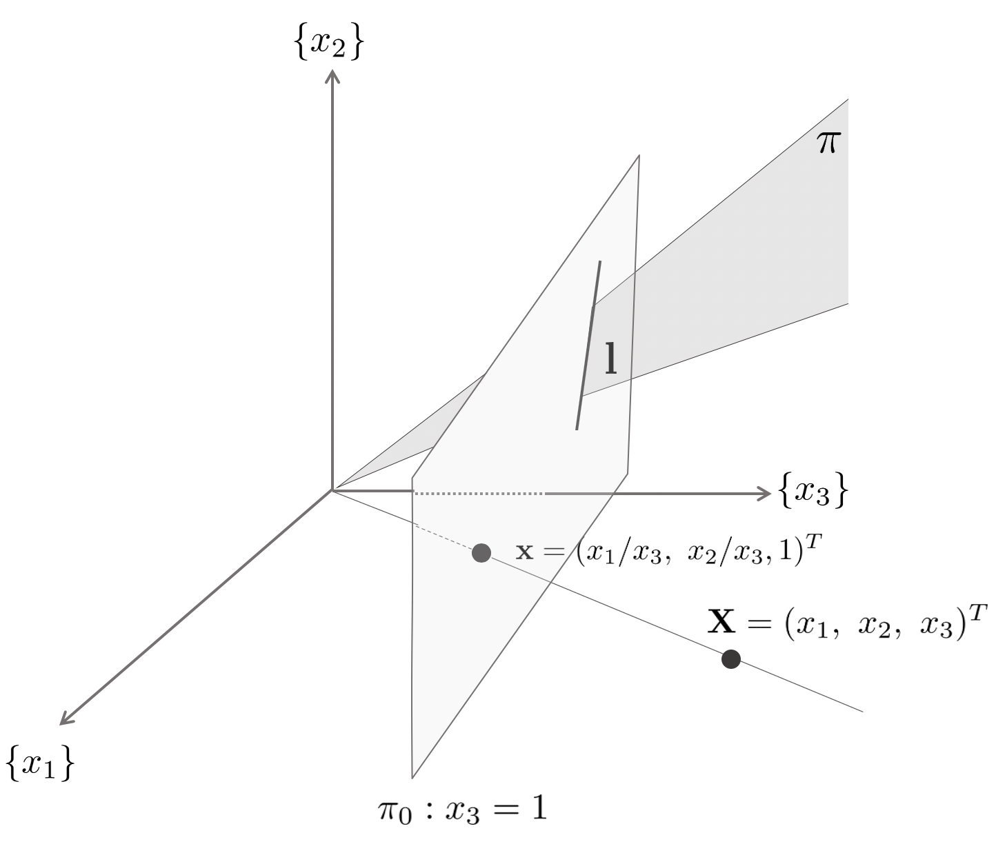
기하학적으로 봤을 때, $\mathbb{P}^{2}$는 3차원 공간 $\mathbb{R}^{3}$에서 원점을 지나는 모든 직선들의 집합 을 의미한다. $\mathbb{P}^{2}$ 상의 모든 벡터를 $k(x_{1},x_{2},x_{3})^{\intercal}$라고 했을 때 $k$ 값에 따라 한 점 $(x_{1},x_{2},x_{3})^{\intercal}$의 위치가 결정된다. $k$는 실수이므로 $k=0$인 경우 원점을 의미하고 $k\neq0$인 경우 무수한 점들의 집합인 직선이 된다. 반대로, 이러한 $\mathbb{R}^{3}$ 공간 상의 원점을 통과하는 한 직선은 $\mathbb{P}^{2}$ 공간 상의 한 점으로 볼 수 있다. 이를 확장하면 $\mathbb{P}^{2}$ 공간 상의 직선 $\mathbf{l}$은 $\mathbb{R}^{3}$ 공간 상의 원점을 포함하는 평면 $\pi$에 대응한다.
$\mathbb{P}^{2}$ 공간에서는 스케일 값에 관계없이 한 점을 유일하게 정의할 수 있으므로 마지막 항 $x_{3}$로 좌표값을 나눈 $(x_{1}/x_{3}, x_{2}/x_{3}, 1)$를 일반적으로 한 점을 표현하는 대표값으로 간주한다. 따라서 $\mathbb{R}^{3}$ 공간 상의 원점을 지나는 직선과 $x_{3}=1$인 평면이 교차하는 점이 곧 $\mathbb{P}^{2}$ 공간 상의 한 점이 된다.
1.2.4. Duality
$\mathbb{P}^{2}$ 공간에서는 점과 직선이 대칭성(duality)을 가진다. 예를 들어 직선 $\mathbf{l}$ 위의 한 점 $\mathbf{x}$은 $\mathbf{x}^{\intercal}\mathbf{l}=0$ 또는 $\mathbf{l}^{\intercal}\mathbf{x}=0$과 같이 두 가지 방법으로 표현할 수 있다. 또한, 두 직선 $\mathbf{l},\mathbf{l}^{\prime}$이 교차하는 한 점은 $\mathbf{x}=\mathbf{l}\times \mathbf{l}^{\prime}$이고 두 점 $\mathbf{x}, \mathbf{x}^{\prime}$을 통과하는 직선 $\mathbf{l}$은 $\mathbf{l} = \mathbf{x}\times \mathbf{x}^{\prime}$으로 표현할 수 있는데 이는 기본적으로 점과 직선의 위치가 바뀌었을 뿐 동일한 공식을 사용한다.
이와 같이 $\mathbb{P}^{2}$ 공간에서는 점과 직선이 동일한 공식에 대해 위치를 바꾸어도 성립하는 대칭성을 가진다. 즉, 두 점을 통과하는 직선의 공식은 두 직선이 교차하는 한 점의 공식과 대칭이다.
1.3. Conics and dual conics
conic이란 평면에서 이차식으로 정의된 곡선을 의미한다. 일반적인 공식으로는
\begin{equation}
\begin{aligned}
ax^{2} + bxy +cy^{2} +dx+ ey + f = 0
\end{aligned}
\end{equation}
과 같으며 계수 값에 따라 원, 타원, 쌍곡선, 포물선 등 다양한 곡선 형태로 표현될 수 있다. conic을 homogeneous form으로 나타내면
\begin{equation}
\begin{aligned}
ax^{2} + bxy +cy^{2} +dxz+ eyz + fz^{2} = 0
\end{aligned}
\end{equation}
과 같고 이를 행렬 형태로 정리하면
\begin{equation}
\begin{aligned}
\begin{pmatrix} x&y&z \end{pmatrix} \begin{pmatrix} a&b/2&d/2 \\ b/2&c&e/2 \\ d/2&e/2&f \end{pmatrix} \begin{pmatrix} x\\y\\z \end{pmatrix} =0
\end{aligned}
\end{equation}
꼴로 쓸 수 있으며 이 때 대칭행렬 $\begin{pmatrix} a&b/2&d/2 \\ b/2&c&e/2 \\ d/2&e/2&f \end{pmatrix}$를 conic $\mathbf{C}$라고 한다.
1.3.1. Five points define a conic
conic $\mathbf{C}$가 유일하게 결정되기 위해서는 다섯개의 점이 필요하다. 하나의 점에 대한 conic 방정식은 다음과 같이 다시 쓸 수 있다.
\begin{equation}
\begin{aligned}
& ax^{2} + bxy +cy^{2} +dxz+ eyz + fz^{2} = 0 \\
& \Rightarrow \begin{pmatrix} x_{i}^{2}&x_{i}y_{i}&y_{i}^{2}&x_{i}&y_{i}&1 \end{pmatrix} \mathbf{c} = 0
\end{aligned}
\end{equation}
이 때, $\mathbf{c} = \begin{pmatrix} a&b&c&d&e&f \end{pmatrix} \in \mathbb{R}^{6}$인 벡터를 의미한다. $\mathbf{c}$는 5 자유도를 가지므로
\begin{equation}
\begin{aligned}
& \underbrace{\begin{bmatrix}
x_{1}^{2}&x_{1}y_{1}&y_{1}^{2}&x_{1}&y_{1}&1 \\
x_{2}^{2}&x_{2}y_{2}&y_{2}^{2}&x_{2}&y_{2}&1 \\
x_{3}^{2}&x_{3}y_{3}&y_{3}^{2}&x_{3}&y_{3}&1 \\
x_{4}^{2}&x_{4}y_{4}&y_{4}^{2}&x_{4}&y_{4}&1 \\
x_{5}^{2}&x_{5}y_{5}&y_{5}^{2}&x_{5}&y_{5}&1 \\
\end{bmatrix}}_{\mathbf{A}} \mathbf{c} = 0
\end{aligned}
\end{equation}
위 식과 같이 총 5개의 점을 사용하면 $\mathbf{A} \in \mathbb{R}^{5\times 6}$ 행렬의 null space 벡터가 유일한 $\mathbf{c}$의 해가 되고 conic을 유일하게 결정한다.
1.3.2. Tangent lines to conics
conic $\mathbf{C}$ 위의 한 점 $\mathbf{x}$에서 접선 $\mathbf{l}$은
\begin{equation}
\begin{aligned}
\mathbf{l} = \mathbf{Cx}
\end{aligned}
\end{equation}
와 같이 쓸 수 있다.
임의의 두 직선 $\mathbf{l},\mathbf{m}$을 포함하는 conic $\mathbf{C}$는
\begin{equation}
\begin{aligned}
\mathbf{C} = \mathbf{l}\mathbf{m}^{\intercal} + \mathbf{m}\mathbf{l}^{\intercal}
\end{aligned}
\end{equation}
과 같이 쓸 수 있다.
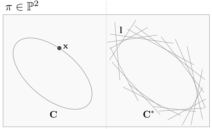
1.3.3. Dual conics
사영 공간(projective space) $\mathbb{P}^{n}$은 $\mathbb{R}^{n+1}$ 공간 상의 원점을 지나는 직선들의 집합을 의미 한다. 이와 대칭을 이루는 dual projective space $(\mathbb{P}^{n})^{\vee}$는 $\mathbb{R}^{n}$ 공간 상 n차원 부분 선형공간들의 집합을 의미한다.
n차원 부분 선형공간 $\mathbf{H}$는
\begin{equation}
\begin{aligned}
\mathbf{H} = \{\sum_{i=0}^{n}a_{i}x_{i}=0 \ | \ a_{i}\neq 0 \ \text{ for some i}\}.
\end{aligned}
\end{equation}
이 때 $a_{0},\cdots,a_{n} \in \mathbb{P}^{n}$을 하나의 사영 공간(projective space)로 생각할 수 있고 하나의 dual projective space는 하나의 사영 공간과 대칭 관계를 가진다.
$\mathbb{P}^{2}$ 상의 conic $\mathbf{C}$가 주어졌을 때, $\mathbf{C}$의 dual conic $\mathbf{C}^{\ast}$은 $(\mathbb{P}^{2})^{\vee}$ 공간 상의 conic을 의미하며 $\mathbf{C}^{\ast}$은 conic $\mathbf{C}$의 접선에 대한 정보를 가지고 있다. $(\mathbb{P}^{2})^{\vee}$는 $\mathbb{P}^{2}$ 상의 직선을 파라미터화하여 나타낼 수 있다. $\hat{\mathbf{C}}^{\ast}$는 다음과 같이 나타낼 수 있다.
\begin{equation}
\begin{aligned}
\mathbf{C}^{\ast}_{ij} = (-1)^{i+j} \det(\hat{\mathbf{C}}_{ij})
\end{aligned}
\end{equation}
여기서 $\hat{\mathbf{C}}_{ij}$는 $\mathbf{C}_{ij}$에서 i번째 행, j번째 열을 제거한 행렬을 의미한다.
임의의 직선 $\mathbf{l}$이 주어졌을 때 $\mathbf{l}$이 conic $\mathbf{C}$에 접하는 필요충분조건은 다음과 같다.
\begin{equation}
\begin{aligned}
\mathbf{l}^{\intercal}\mathbf{C}^{\ast}\mathbf{l} = 0
\end{aligned}
\end{equation}
1.3.4. Proof
($\Rightarrow$) conic $\mathbf{C} \in \mathbb{R}^{3\times 3}$의 rank가 3이고 non-singular하다고 가정하면 $\mathbf{C}^{\ast} = \det(\mathbf{C}^{-1})$와 같이 나타낼 수 있다. $\mathbf{C}$ 위의 한 점 $\mathbf{x} \in \mathbf{C}$가 주어졌을 때 $\mathbf{x}$에서 접선 $\mathbf{l}$은 $\mathbf{l} = \mathbf{Cx}$로 나타낼 수 있다. 이를 위 식에 대입하면
\begin{equation}
\begin{aligned}
\mathbf{l}^{\intercal}\mathbf{C}^{\ast}\mathbf{l} & = (\mathbf{Cx})^{\intercal}\mathbf{C}^{\ast}\mathbf{Cx} \\
& = \mathbf{x}^{\intercal}\mathbf{C}^{\intercal}\mathbf{C}^{\ast}\mathbf{Cx} \\
& = \det(\mathbf{x}^{\intercal}\mathbf{C}^{\intercal}\mathbf{x}) & \because \mathbf{C}^{\ast}=\det(\mathbf{C}^{-1}) \\
& = 0 & \because \mathbf{x} \in \mathbf{C}, (\mathbf{x}^{\intercal}\mathbf{C}\mathbf{x})^{\intercal} = 0
\end{aligned}
\end{equation}
($\leftarrow$) 직선 $\mathbf{l}$과 dual conic $\mathbf{C}^{\ast}$가 $\mathbf{l}^{\intercal}\mathbf{C}^{\ast}\mathbf{l}=0$을 만족할 때 $\mathbf{l}$과 $\mathbf{C}^{\ast}$가 한 점 $\mathbf{x}$에서 만난다는 것을 증명하면 된다. 이 때 $\mathbf{l} = \mathbf{Cx}$ 공식이 성립한다.
$\mathbf{C}$는 non-singualr하기 때문에 역행렬이 존재하므로 $\mathbf{x} = \mathbf{C}^{-1}\mathbf{l}$과 같이 나타낼 수 있다. 따라서 $\mathbf{x}^{\intercal}\mathbf{l}$은
\begin{equation}
\begin{aligned}
\mathbf{x}^{\intercal}\mathbf{l} & = (\mathbf{C}^{-1}\mathbf{l})^{\intercal}\mathbf{l} \\
& = \mathbf{l}^{\intercal}\mathbf{C}^{-t}\mathbf{l} = 0 \\
& (\mathbf{C}^{\ast} \sim \mathbf{C}^{-1} \ \text{ by assumption.}) \\
\end{aligned}
\end{equation}
과 같고 $\mathbf{x}^{\intercal}\mathbf{Cx}$는
\begin{equation}
\begin{aligned}
\mathbf{x}^{\intercal}\mathbf{C}\mathbf{x} & = (\mathbf{C}^{-1}\mathbf{l})^{\intercal}\mathbf{C}\mathbf{C}^{-1}\mathbf{l} \\
& = \mathbf{l}^{\intercal}\mathbf{C}^{-t}\mathbf{cc}^{-1}\mathbf{l} \\
& = \mathbf{l}^{\intercal}\mathbf{C}^{-1}\mathbf{l} = 0 \\
& (\mathbf{C}^{-t} = \mathbf{C}^{-1} \ \ \mathbf{C} \text{ is symmetric.})
\end{aligned}
\end{equation}
공식이 성립함에 따라 $\mathbf{x}$는 $\mathbf{l}$과 $\mathbf{C}$의 교점임이 증명된다.
\begin{equation}
\begin{aligned}
\{\mathbf{x}\} = \mathbf{l} \cap \mathbf{C}
\end{aligned}
\end{equation}
1.4. Projective transformations
$\mathbb{P}^{2}$의 projective transformation은 non-singular인 $3\times3$ 행렬로 정의되는 $\mathbb{P}^{2} \Rightarrow \mathbb{P}^{2}$ 사상을 의미하며 직선을 직선으로 보내는 성질을 가진다. projective transformation은 collineation, projectivity 또는 homography 라고도 불린다.
1.5. A hierarchy of transformations
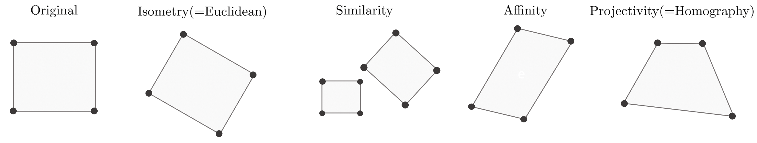
projective 변환은 변환 전과 후 사이에 어떤 성질을 보존하느냐에 따라 여러 종류의 변환 행렬이 존재한다.
1.5.1. Class 1: isometries
물체가 변환 전과 후 사이에 물체의 크기가 동일한 경우 해당 변환을 isometry 변환이라고 부른다.
\begin{equation}
\begin{aligned}
\mathbf{H}_{iso} = \begin{bmatrix} \mathbf{A}&\mathbf{t} \\ \mathbf{0} & 1 \end{bmatrix}
\end{aligned}
\end{equation}
이 때 $\mathbf{A} \in \mathbb{R}^{2\times2}$는 2차원 물체의 회전과 반사(reflection)을 포함한 행렬이며 $\mathbf{t} \in \mathbb{R}^{2}$는 2차원 물체의 이동 벡터이다.
1.5.2. Class 2: similarity transformations
isometry 변환에 스케일을 의미하는 $s$가 추가된 변환을 similarity 변환이라고 하며 물체의 이동 및 회전에 추가적으로 스케일까지 같이 변환하는 성질을 가진다. 이 때 기존의 $\mathbf{A}$ 행렬에서 reflection의 성질을 제거한 $\mathbf{R}$ 행렬을 사용한다.
\begin{equation}
\begin{aligned}
\mathbf{H}_{S} = \begin{bmatrix} s\mathbf{R}&\mathbf{t} \\ \mathbf{0} & 1 \end{bmatrix}
\end{aligned}
\end{equation}
similarity 변환은 물체의 각도와 길이의 비율을 보존되지만 스케일은 보존되지 않는다. 두 물체가 similarity 변환까지 동일하다는 의미는(=up to scale) 두 물체의 형태는 동일하지만 스케일에 차이가 있다는 의미이다.
1.5.3. Class 3: affine transformations
affine 변환은 isometry 변환에서 행렬 $\mathbf{A}$의 아무 제약조건이 없는 변환행렬을 의미한다. 변환 후 물체는 일반적으로 변환 전과 다른 형태를 가진다.
\begin{equation}
\begin{aligned}
\mathbf{H}_{A} = \begin{bmatrix} \mathbf{A}&\mathbf{t} \\ \mathbf{0} & 1 \end{bmatrix}
\end{aligned}
\end{equation}
$\mathbf{H}_{A}$는 6자유도를 가지므로 세 개의 대응점 쌍으로부터 $\mathbf{H}_{A}$를 유일하게 결정할 수 있다.
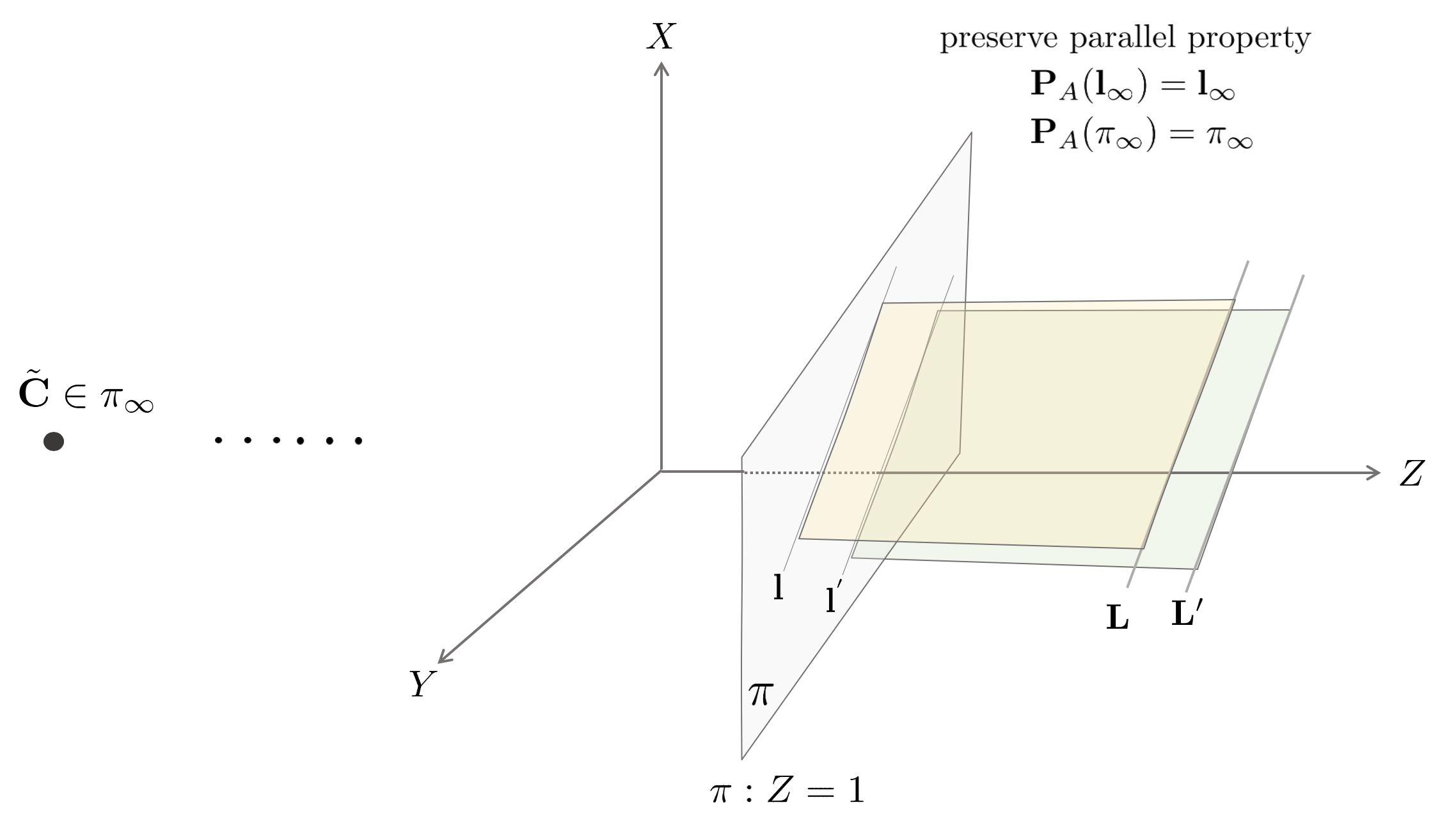
affine 변환은 물체의 길이 비율을 보존하며 또한 평행한 직선을 보존하는 성질을 가진다. 따라서 무한대 직선(line at infinity) $\mathbf{l}_{\infty}$를 affine 변환해도 여전히 $\mathbf{l}_{\infty}$가 된다.
\begin{equation}
\begin{aligned}
\mathbf{H}_{A}(\mathbf{l}_{\infty}) = \mathbf{l}_{\infty}
\end{aligned}
\end{equation}
1.5.4. Class 4: projective transformations
마지막으로 projective 변환은 변환행렬의 마지막 행이 $(0,0,1)$이 아닌 임의의 형태를 가지는 변환행렬을 의미한다. projective 변환은 직선을 직선으로 사상한다는 성질 외에는 이전에 설명한 모든 성질들을 보존하지 않는다는 특징이 있다. 평행한 직선 또한 projective 변환을 수행하면 평행하지 않게되며 물체의 길이비 또한 달라지게 된다.
\begin{equation}
\begin{aligned}
\mathbf{H}_{P} = \begin{bmatrix} \mathbf{A}&\mathbf{t} \\ \mathbf{v}^{\intercal}&v\end{bmatrix}
\end{aligned}
\end{equation}
이 때 $\mathbf{v}=\begin{bmatrix} v_{1}&v_{2} \end{bmatrix}^{\intercal}$는 임의의 2차원 벡터를 의미하며 $v$ 또한 임의의 스칼라 값을 의미한다. projective 변환행렬 $\mathbf{H}_{P}$는 8자유도를 가지므로 일반적으로 4개의 대응점 쌍을 통해 $\mathbf{H}_{P}$을 유일하게 결정할 수 있다.
1.6. Decomposition of a projective transformation
앞서 설명한 변환행렬의 계층구조에 따라 projective 변환행렬은 다른 변환행렬들의 곱으로 표현할 수 있다. 반대로 말하면, projective 변환은 다른 변환행렬들로 분해가 가능하다. 임의의 projective 변환 $\mathbf{H}_{p}$가 주어졌을 때
\begin{equation}
\begin{aligned}
\mathbf{H}_{p} & = \mathbf{H}_{S}\mathbf{H}_{A}\mathbf{H}_{P} \\
& = \begin{bmatrix} s \mathbf{R}&\mathbf{t} \\\mathbf{0}&1 \end{bmatrix} \begin{bmatrix} \mathbf{K} & \mathbf{0} \\ \mathbf{0} & 1 \end{bmatrix} \begin{bmatrix} \mathbf{I} & \mathbf{0}\\ \mathbf{v}^{\intercal}& v\end{bmatrix} \\
& = \begin{bmatrix} \mathbf{A}&\mathbf{t} \\ \mathbf{v}^{\intercal}&v \end{bmatrix}
\end{aligned}
\end{equation}
와 같이 projective 변환 $\mathbf{H}_{p}$는 similarity 변환 $\mathbf{H}_{S}$과 affine 변환 $\mathbf{H}_{A}$ 그리고 나머지 변환 $\mathbf{H}_{P}$의 곱으로 분해가 가능하다. 이 때, $\mathbf{A}=s\mathbf{R}\mathbf{K}+\mathbf{tv}^{\intercal}$이고 $\mathbf{K}$는 $\det(\mathbf{K})=1$로 정규화된 상삼각행렬(upper-triangle) 행렬을 의미한다. 단, 위와 같은 분해는 $v \neq 0$일 때만 가능하며 $s >0$인 경우 분해가 유일하게 결정된다.
$\mathbf{H}^{-1} = \mathbf{H}_{P}^{-1}\mathbf{H}_{A}^{-1}\mathbf{H}_{S}^{-1} = \mathbf{H}_{P}'\mathbf{H}_{A}'\mathbf{H}_{S}'$ 또한 $\mathbf{H}$의 반대 방향으로 homography 연산을 의미한다. 이 때, 각 행렬의 디테일한 $\mathbf{R},\mathbf{t},\mathbf{K},\mathbf{v}, s, v$ 값은 $\mathbf{H}$와 $\mathbf{H}^{-1}$이 서로 다르다.
1.7. Recovery of affine and metric properties from images
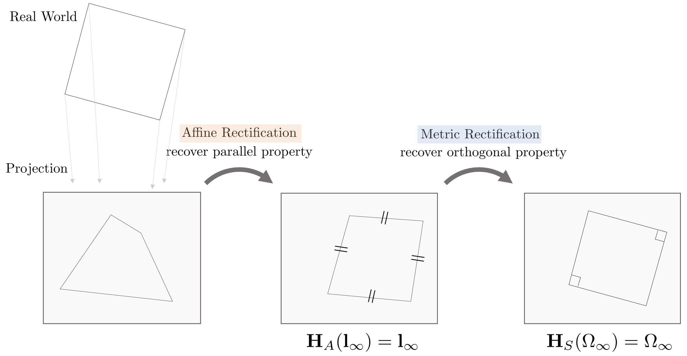
임의의 이미지가 주어졌을 때 이미지 상에서 평행한 선들과 직교한 선들을 사용하여 affine 성질과 metric 성질을 복원할 수 있다.
1.7.1. The line at infinity
Affine 변환은 평행한 선들이 보존되는 Affine 성질을 보존하는 것을 의미하며 무한대 직선(line at infinity) $\mathbf{l}_{\infty} = \begin{bmatrix} 0&0&1 \end{bmatrix}^{\intercal}$을 Affine 변환해도 여전히 무한대 직선의 성질을 유지하는 특징이 있다.
\begin{equation}
\begin{aligned}
\mathbf{H}_{A}(\mathbf{l}_{\infty}) = \mathbf{H}_{A}^{-\intercal}\mathbf{l}_{\infty} =\begin{bmatrix} \mathbf{A}&\mathbf{t} \\0&1 \end{bmatrix}^{-\intercal} \begin{bmatrix} 0\\0\\1 \end{bmatrix} = \begin{bmatrix} \mathbf{A}^{-\intercal}&0 \\-\mathbf{t}^{\intercal}\mathbf{A}^{-\intercal} &1 \end{bmatrix} \begin{bmatrix} 0 \\ 0 \\ 1 \end{bmatrix} = \begin{bmatrix} 0 \\ 0 \\ 1 \end{bmatrix} = \mathbf{l}_{\infty}^{\prime}
\end{aligned}
\end{equation}
위와 같이 $\mathbf{l}_{\infty}$를 Affine 변환해도 여전히 무한대에 위치한다.
1.7.2. Recovery of affine properties from images
affine 성질을 복원한다는 의미는 실제 세계에서 평행하지만 이미지 평면상에서 projective 변환에 의해 평행하지 않은 두 직선을 다시 복원한다는 의미이다. 임의의 homography $\mathbf{H}$가 affine 성질을 보존한다는 의미는 곧 무한대 직선 $\mathbf{l}_{\infty}$를 $\mathbf{H}$ 변환해도 무한대에 위치한 직선이 된다는 의미이다. 즉, 무한대 직선 위의 한 점 $\mathbf{x}_{\infty}$ 점이 있다고 했을 때 다음이 성립한다.
\begin{equation}
\begin{aligned}
\mathbf{H}(\mathbf{x}_{\infty}) = \mathbf{Hx}_{\infty} = \mathbf{x}_{\infty}^{\prime}
\end{aligned}
\end{equation}
무한대 직선 위의 한 점 $\mathbf{x}_{\infty}$는 $\mathbf{x}_{\infty}=(x,y,0)^{\intercal}$와 같이 마지막 항이 0인 특징이 있으므로 임의의 homography $\mathbf{H}$는
\begin{equation}
\begin{aligned}
\mathbf{H}\mathbf{x}_{\infty} = \begin{bmatrix} \mathbf{A}& \mathbf{t} \\ \mathbf {v} & v \end{bmatrix} \begin{bmatrix} x\\y\\0 \end{bmatrix} = \begin{bmatrix} *\\ * \\0 \end{bmatrix}
\end{aligned}
\end{equation}
이 성립하므로 $\mathbf{v}=(0,0)$이 되고 $v$는 스케일 상수가 되어 1로 변환이 가능하다.
\begin{equation}
\begin{aligned}
\mathbf{H} = \begin{bmatrix} \mathbf{A}&\mathbf{t} \\ \mathbf{0} & v \end{bmatrix} = \begin{bmatrix} \mathbf{A}/v & \mathbf{t}/v \\ \mathbf{0} & 1 \end{bmatrix}
\end{aligned}
\end{equation}
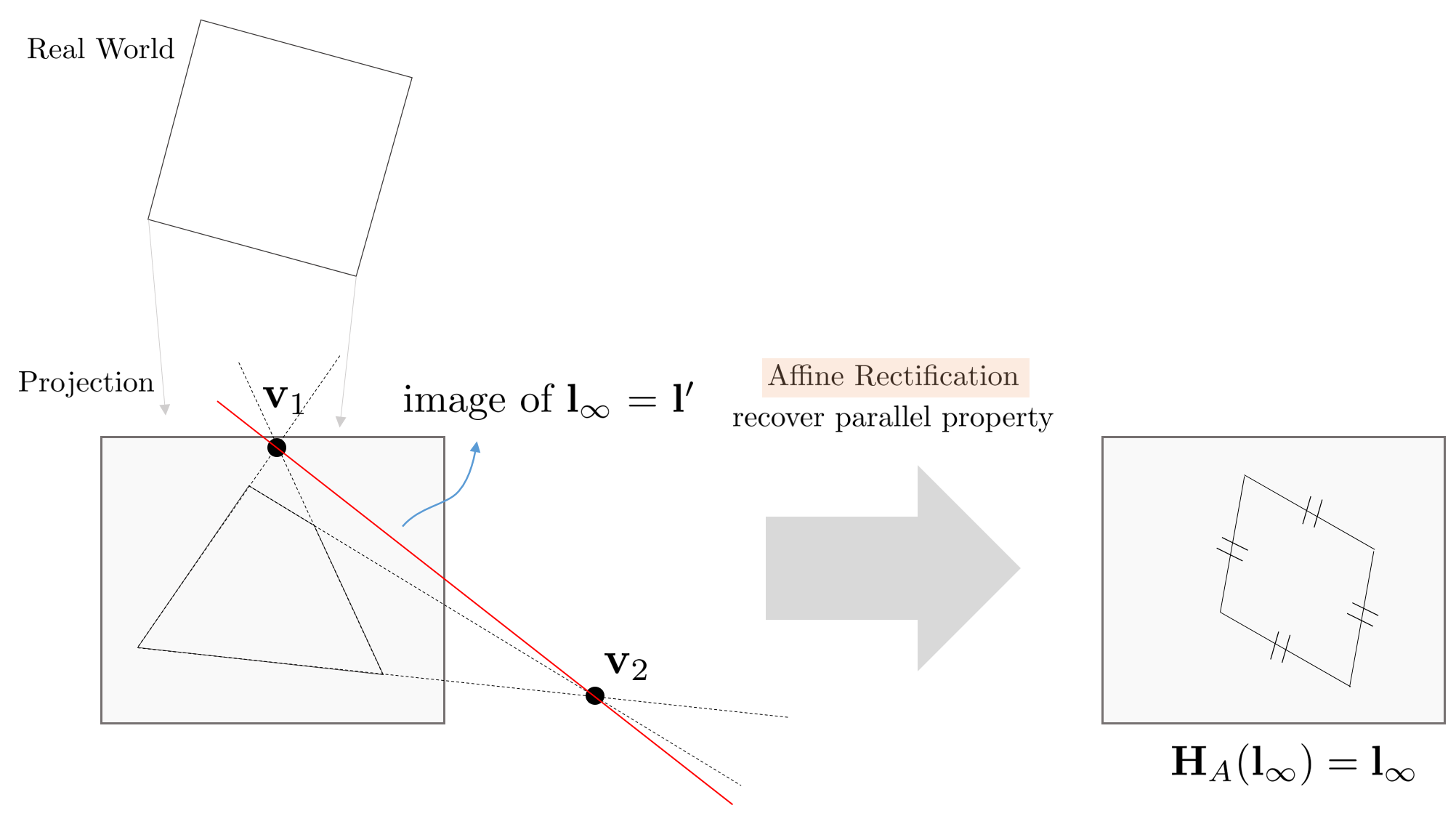
하지만 현실의 카메라를 통해 촬영한 영상에서는 projective 변환이 적용되므로 $\mathbf{l}_{\infty}$의 성질이 보존되지 않고 이미지 상에 투영된다. 따라서 이미지 상에 투영된 임의의 직선 $\mathbf{l}^{'}$을 $\mathbf{l}_{\infty}$로 변환하는 homography $\mathbf{H}$를 찾는 과정이 affine rectification이 된다.
\begin{equation}
\begin{aligned}
\mathbf{H}(\mathbf{l}^{'}) = \mathbf{H}^{-\intercal}\mathbf{l}^{'} = \mathbf{l}_{\infty}
\end{aligned}
\end{equation}
임의의 한 직선은 $\mathbf{l}^{'}=\begin{bmatrix} a & b & c \end{bmatrix}^{\intercal}$와 같이 나타낼 수 있고 $\mathbf{l}_{\infty}=\begin{bmatrix} 0 & 0 & 1 \end{bmatrix}^{\intercal}$ 이므로 이를 다시 표현하면 다음과 같다.
\begin{equation}
\begin{aligned}
\mathbf{H}(\mathbf{l}^{'}) = \mathbf{H}^{-\intercal}\begin{bmatrix} a \\ b \\ c \end{bmatrix}=\begin{bmatrix} 0 \\ 0 \\ 1 \end{bmatrix}
\end{aligned}
\end{equation}
다음으로 $\mathbf{H}$의 성분을 찾아야 한다. projective 변환은 다음과 같이 3개로 분리할 수 있고
\begin{equation}
\begin{aligned}
\mathbf{H}_{p} & = \mathbf{H}_{S}\mathbf{H}_{A}\mathbf{H}_{P} \\
& = \begin{bmatrix} s \mathbf{R}&\mathbf{t} \\\mathbf{0}&1 \end{bmatrix} \begin{bmatrix} \mathbf{K} & \mathbf{0} \\ \mathbf{0} & 1 \end{bmatrix} \begin{bmatrix} \mathbf{I} & \mathbf{0}\\ \mathbf{v}^{\intercal}& v\end{bmatrix} \\
& = \begin{bmatrix} \mathbf{A}&\mathbf{t} \\ \mathbf{v}^{\intercal}&v \end{bmatrix}
\end{aligned}
\end{equation}
이 중, $\mathbf{H}_{P}$ 변환이 $\mathbf{l}_{\infty}$ 성질을 보존하지 않는 projective 변환의 성질을 지닌다. 따라서 $\mathbf{H}$의 형태는 다음과 같다.
\begin{equation}
\begin{aligned}
\mathbf{H} = \begin{bmatrix} \mathbf{I} & \mathbf{0}\\ \mathbf{v}^{\intercal}& v\end{bmatrix}
\end{aligned}
\end{equation}
위 형태를 만족하면서 $\mathbf{l}^{'}$를 $\mathbf{l}_{\infty}$로 변환시키는 $\mathbf{H}$는 다음과 같다.
\begin{equation}
\begin{aligned}
\mathbf{H} = \begin{bmatrix} 1 & 0 & 0 \\ 0 & 1 & 0 \\ a & b & c\end{bmatrix}
\end{aligned}
\end{equation}
\begin{equation}
\begin{aligned}
\mathbf{H}^{-\intercal}\mathbf{l}^{'} = \mathbf{l}_{\infty} = \begin{bmatrix} 1 & 0 & 0 \\ 0 & 1 & 0 \\ a & b & c\end{bmatrix}^{-\intercal}\begin{bmatrix} a \\ b \\ c \end{bmatrix}=\begin{bmatrix} 0 \\ 0 \\ 1 \end{bmatrix}
\end{aligned}
\end{equation}
지금까지 affine rectification 순서를 정리하면 다음과 같다.
1. 실제 세계에서 평행한 직선 2쌍의 좌표를 구한다.
2. 평행한 직선 1쌍 당 소실점(=image of point at infinity) $\mathbf{v}$를 구한다. 총 2쌍이므로 2개 $\mathbf{v}_{1}, \mathbf{v}_{2}$를 구한다.
3. $\mathbf{v}_{1}$, $\mathbf{v}_{2}$를 잇는 image of line at infinity $\mathbf{l}^{'} = [a,b,c]^{\intercal}$를 구한다.
4. $\mathbf{l}^{'}$를 바탕으로 recover homography $\mathbf{H}$를 구한다.
\begin{equation}
\begin{aligned}
\mathbf{H} = \begin{bmatrix} 1 & 0 & 0 \\ 0 & 1 & 0 \\ a & b & c\end{bmatrix}
\end{aligned}
\end{equation}
5. 이미지 전체에 $\mathbf{H}$를 적용하여 affine rectification을 마무리한다. affine rectification 결과 이미지는 평행한 선들이 보존된다.
1.7.3. Recovery of metric properties from images
metric성질을 복원한다는 의미는 실제 세계에서 수직이지만 이미지 평면상에서 projective 변환에 의해 직교하지 않은 두 직선을 다시 복원한다는 의미이다. 이 때, 복원된 이미지는 정확한 스케일 값까지는 알 수 없다(up to similarity, up to scale). 즉, metric rectification은 원본 이미지와 스케일 값만 다른 영상까지 복원한다는 의미이다. 이를 수행하기 위해서는 absolute dual conic $\mathbf{C}_{\infty}^{\ast}$의 특징을 사용하여 복원해야 한다.
Circular Point
circular point (또는 absolute point) $\mathbf{x}_{c}, \mathbf{x}_{-c}$는 다음과 같이 정의된다.
\begin{equation}
\begin{aligned}
\mathbf{x}_{\pm c} = \begin{bmatrix} 1 \\ \pm i \\ 0 \end{bmatrix} \in \mathbb{CP}^{2}
\end{aligned}
\end{equation}
- $i = \sqrt{-1}$
- $\mathbb{CP}^{2}$ : complex projective space
임의의 homography $\mathbf{H}$가 circular point 집합을 보존하면 $\mathbf{H}$는 simliarity 성질을 보존하는 특징이 있다.
\begin{equation}
\begin{aligned}
\mathbf{H}(\mathbf{x}_{\pm c}) = \mathbf{x}_{\pm c} \quad \text{then, } \mathbf{H} \in \mathbf{H}_{s}
\end{aligned}
\end{equation}
따라서 $\mathbf{H}$의 형태는 다음과 같다.
\begin{equation}
\begin{aligned}
\mathbf{H} = \begin{bmatrix} A & t \\ 0 & 1 \end{bmatrix} = \begin{bmatrix} s\mathbf{R} & t \\ 0 & 1 \end{bmatrix}
\end{aligned}
\end{equation}
- $s$ : scale factor
- $\mathbf{R}$ : rotation matrix
Dual Conic Properties
$\mathbb{P}^{2}$ 공간 상의 두 점 $\mathbf{P}$, $\mathbf{Q}$가 존재할 때 두 점을 잇는 직선에 접하는 dual conic $\mathbf{C}^{\ast}$는 다음과 같이 나타낼 수 있다.
\begin{equation}
\begin{aligned}
\mathbf{C}^{\ast} = \mathbf{P}\mathbf{Q}^{\intercal} + \mathbf{Q}\mathbf{P}^{\intercal}
\end{aligned}
\end{equation}
- $\mathbf{P} = [p_1, p_2, p_3]^{\intercal}$
이 때, $\mathbf{C}^{\ast}$는 두 점 $\mathbf{P}$와 $\mathbf{Q}$를 지나는 직선 $\mathbf{l}$을 매개화하는 dual conic을 의미한다. dual conic과 $\mathbf{C}^{\ast}$과 이에 접하는 직선 $\mathbf{l}$은 다음과 같은 관계를 가진다.
\begin{equation}
\begin{aligned}
\mathbf{l}^{\intercal}\mathbf{C}^{\ast}\mathbf{l} = 0
\end{aligned}
\end{equation}
\begin{equation}
\begin{aligned}
\mathbf{l}^{\intercal}(\mathbf{P}\mathbf{Q}^{\intercal} + \mathbf{Q}\mathbf{P}^{\intercal})\mathbf{l} = 0
\end{aligned}
\end{equation}
직선 $\mathbf{l}$ 상에 두 점 $\mathbf{P}$와 $\mathbf{Q}$가 포함되므로 $\mathbf{P}^{\intercal}\mathbf{l}=0$ 또는 $\mathbf{Q}^{\intercal}\mathbf{l}=0$ 이 성립하여 위 식이 만족된다.
Absolute Dual Conic
absolute dual conic $\mathbf{C}^{\ast}_{\infty}$은 두 개의 circular point를 지나는 직선을 매개화하는 dual conic을 의미한다.
\begin{equation}
\begin{aligned}
\mathbf{C}^{\ast}_{\infty} = \mathbf{x}_{c}\mathbf{x}_{-c}^{\intercal} + \mathbf{x}_{-c}\mathbf{x}_{c}^{\intercal}
\end{aligned}
\end{equation}
\begin{equation}
\begin{aligned}
\mathbf{C}^{\ast}_{\infty} & = \begin{bmatrix} 1 \\ i \\ 0 \end{bmatrix}\begin{bmatrix} 1 & -i & 0 \end{bmatrix} + \begin{bmatrix} 1 \\ -i \\ 0 \end{bmatrix}\begin{bmatrix} 1 & i & 0 \end{bmatrix} \\
& = \begin{bmatrix} 1 & 0 & 0 \\ 0 & 1 & 0 \\ 0 & 0 & 0 \end{bmatrix}
\end{aligned}
\end{equation}
$\mathbb{P}^{2}$ 공간 상의 임의의 두 직선 $\mathbf{l}, \mathbf{l}'$ 이 존재할 때 두 직선의 각도는 다음과 같이 나타낼 수 있다.
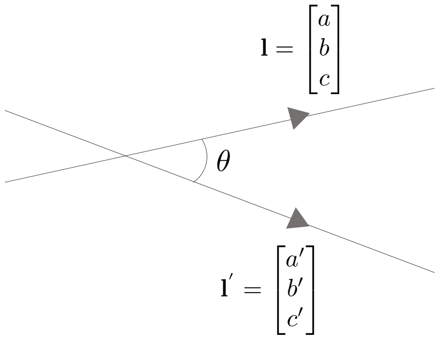
\begin{equation}
\begin{aligned}
\cos\theta = \frac{aa' + bb'}{\sqrt{a^{2} + b^{2}}\sqrt{a'^{2} + b'^{2}}}
\end{aligned}
\end{equation}
이 때, 위 식을 $\mathbf{C}^{\ast}_{\infty} = \begin{bmatrix} 1 & 0 & 0 \\ 0 & 1 & 0 \\ 0 & 0 & 0 \end{bmatrix}$를 사용하여 표현하면 다음과 같다.
\begin{equation}
\begin{aligned}
\cos\theta = \frac{ \mathbf{l}^{\intercal}\mathbf{C}_{\infty}^{\ast}\mathbf{l}' }{ \sqrt{\mathbf{l}^{\intercal}\mathbf{C}_{\infty}^{\ast}\mathbf{l}} \sqrt{\mathbf{l}'^{\intercal}\mathbf{C}_{\infty}^{\ast}\mathbf{l}'} }
\end{aligned}
\end{equation}
- $aa' + bb' = \mathbf{l}^{\intercal}\mathbf{C}_{\infty}^{\ast}\mathbf{l}'$
- $\sqrt{a^{2} + b^{2}} = \sqrt{\mathbf{l}^{\intercal}\mathbf{C}_{\infty}^{\ast}\mathbf{l}}$
- $\sqrt{a'^{2} + b'^{2}} = \sqrt{\mathbf{l}'^{\intercal}\mathbf{C}_{\infty}^{\ast}\mathbf{l}'}$
Homography of Dual Conic
dual conic과 $\mathbf{C}^{\ast}$과 이에 접하는 직선 $\mathbf{l}$은 다음과 같은 관계를 가진다.
\begin{equation}
\begin{aligned}
\mathbf{l}^{\intercal}\mathbf{C}^{\ast}\mathbf{l} = 0
\end{aligned}
\end{equation}
앞서 설명한 위 공식에 Homography $\mathbf{H}: \mathbb{P}^{2} \mapsto \mathbb{P}^{2}$를 수행하면 다음과 같다. $\mathbf{H}(\mathbf{l}) = \mathbf{H}^{-\intercal}\mathbf{l}$이므로
\begin{equation}
\begin{aligned}
(\mathbf{H}^{-\intercal}\mathbf{l})^{\intercal} \mathbf{H}(\mathbf{C}^{\ast}) (\mathbf{H}^{-\intercal}\mathbf{l}) = 0
\end{aligned}
\end{equation}
\begin{equation}
\begin{aligned}
\therefore \mathbf{H}(\mathbf{C}^{\ast}) = \mathbf{H}\mathbf{C}^{\ast}\mathbf{H}^{\intercal}
\end{aligned}
\end{equation}
이 때, $\mathbf{H}(\mathbf{C}^{\ast})$를 image of absolute dual conic $\mathbf{w}$라고 한다.
Image of Absolute Dual Conic
만약 $\mathbb{P}^{2}$ 공간 상에서 두 직선 $\mathbf{l}, \mathbf{m}$이 직교하면 다음과 같은 공식이 성립한다.
\begin{equation}
\begin{aligned}
\mathbf{l}^{\intercal}\mathbf{w}\mathbf{m} = 0
\end{aligned}
\end{equation}
- $\mathbf{w}$ : image of absolute conic $\mathbf{C}_{\infty}^{\ast}$
$\mathbf{w} = \mathbf{H}\mathbf{C}^{\ast}\mathbf{H}^{\intercal}$이므로 $\mathbf{H}$의 형태를 알기 위해 임의의 projective homography $\mathbf{H}$를 분해해보면 다음과 같다.
\begin{equation}
\begin{aligned}
\mathbf{H} & = \mathbf{H}_{S}\mathbf{H}_{A}\mathbf{H}_{P} \\
& = \begin{bmatrix} s \mathbf{R}&\mathbf{t} \\\mathbf{0}&1 \end{bmatrix} \begin{bmatrix} \mathbf{K} & \mathbf{0} \\ \mathbf{0} & 1 \end{bmatrix} \begin{bmatrix} \mathbf{I} & \mathbf{0}\\ \mathbf{v}^{\intercal}& v\end{bmatrix} \\
\end{aligned}
\end{equation}
$\mathbf{H}^{-1} = \mathbf{H}_{P}^{-1}\mathbf{H}_{A}^{-1}\mathbf{H}_{S}^{-1} = \mathbf{H}_{P}'\mathbf{H}_{A}'\mathbf{H}_{S}'$ 또한 동일한 homography 연산을 의미한다. 편의상 $\mathbf{H}_{P}'\mathbf{H}_{A}'\mathbf{H}_{S}'$을 $\mathbf{H}_{P}\mathbf{H}_{A}\mathbf{H}_{S}$라고 표기한다. 이 때, 각 행렬의 디테일한 $\mathbf{R},\mathbf{t},\mathbf{K},\mathbf{v}, s, v$ 값은 $\mathbf{H}$와 $\mathbf{H}^{-1}$이 서로 다르다. 따라서 $\mathbf{H}$의 decompose 순서를 반대로하여 곱해주어 $\mathbf{w}$를 전개해보면 다음과 같다.
\begin{equation}
\begin{aligned}
\mathbf{H}\mathbf{C}^{\ast}\mathbf{H}^{\intercal} = \mathbf{H}_{P}\mathbf{H}_{A}\mathbf{H}_{S} \begin{bmatrix} 1&0&0 \\ 0&1&0 \\ 0&0&0 \end{bmatrix} \mathbf{H}_{S}^{\intercal}\mathbf{H}_{A}^{\intercal}\mathbf{H}_{P}^{\intercal}
\end{aligned}
\end{equation}
\begin{equation}
\begin{aligned}
\mathbf{H}\mathbf{C}^{\ast}\mathbf{H}^{\intercal} = \mathbf{H}_{P}\mathbf{H}_{A} \begin{bmatrix} 1&0&0 \\ 0&1&0 \\ 0&0&0 \end{bmatrix} \mathbf{H}_{A}^{\intercal}\mathbf{H}_{P}^{\intercal}
\end{aligned}
\end{equation}
- $\because \mathbf{H}_{S} \begin{bmatrix} 1&0&0 \\ 0&1&0 \\ 0&0&0 \end{bmatrix} \mathbf{H}_{S}^{\intercal} = \begin{bmatrix} 1&0&0 \\ 0&1&0 \\ 0&0&0 \end{bmatrix}$
이를 전개하면 다음과 같다.
\begin{equation}
\begin{aligned}
\mathbf{w} = \begin{bmatrix} \mathbf{KK}^{\intercal} & \mathbf{KK}^{\intercal}\mathbf{v} \\ \mathbf{v}^{\intercal}\mathbf{K}^{\intercal}\mathbf{K} & \mathbf{v}^{\intercal}\mathbf{KK}^{\intercal}\mathbf{v} \end{bmatrix}
\end{aligned}
\end{equation}
최종적으로 projective 변환이 없는 similarity 변환이라고 가정하면 $\mathbf{v} = 0$이 되고 $\mathbf{w}$는 다음과 같다.
\begin{equation}
\begin{aligned}
\mathbf{w} = \begin{bmatrix} \mathbf{KK}^{\intercal} & 0 \\ 0 & 0 \end{bmatrix}
\end{aligned}
\end{equation}
Metric Rectification
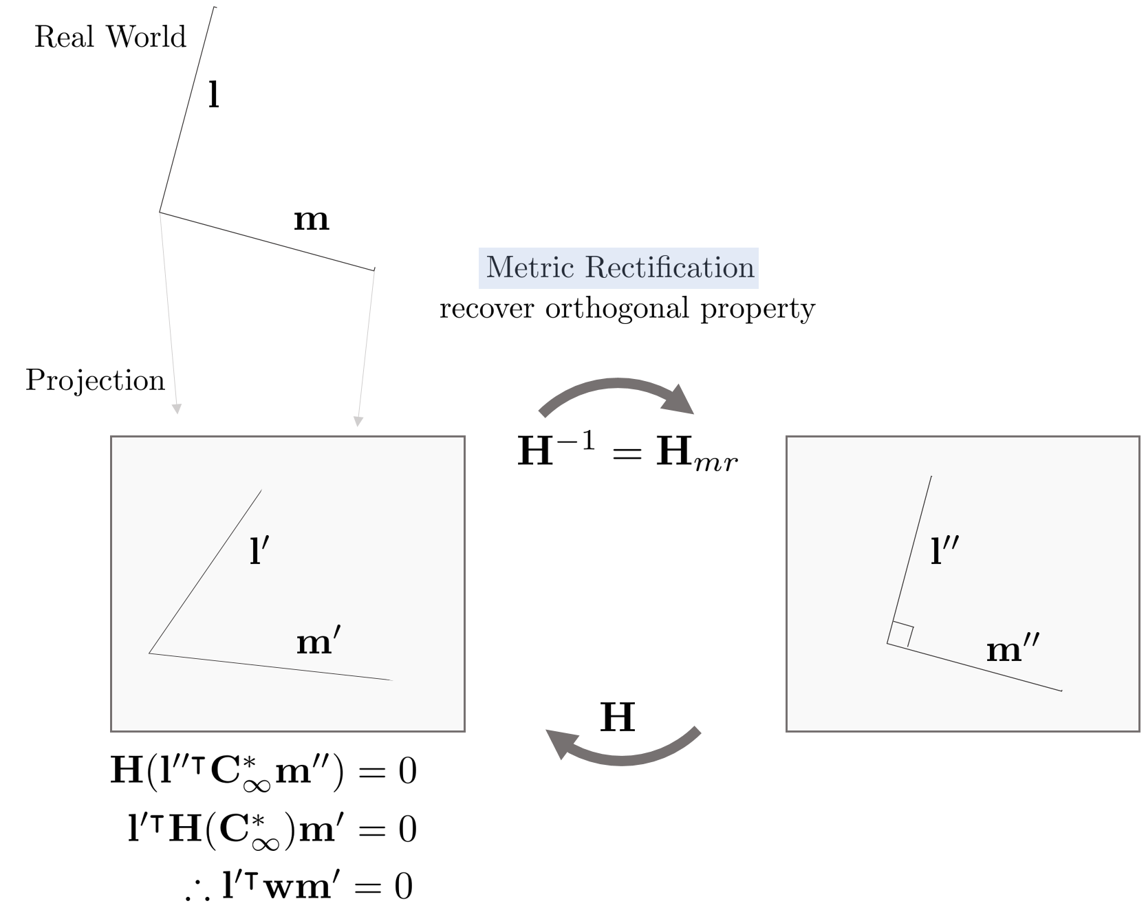
앞서 언급한 내용과 같이 $\mathbf{H}$에 의한 image of absolute dual conic은 $\mathbf{w} = \begin{bmatrix} \mathbf{KK}^{\intercal} & 0 \\ 0 & 0 \end{bmatrix}$로 나타낼 수 있다. 따라서 위 그림에서 $\mathbf{l}''$, $\mathbf{m}''$에 homography 변환 $\mathbf{H}$를 적용한 결과는 다음과 같이 나타낼 수 있다.
\begin{equation}
\begin{aligned}
\mathbf{H}(\mathbf{l}''\mathbf{C}^{\ast}_{\infty}\mathbf{m}'') = \mathbf{l}'\mathbf{w}\mathbf{m}' = 0
\end{aligned}
\end{equation}
- $\mathbf{H}(\mathbf{l}'') = \mathbf{l}'$
- $\mathbf{H}(\mathbf{C}_{\infty}^{\ast}) = \mathbf{w}$
- $\mathbf{H}(\mathbf{m}'') = \mathbf{m}'$
이를 다시 전개하면
\begin{equation}
\begin{aligned}
\mathbf{l}'\begin{bmatrix} \mathbf{KK}^{\intercal} & 0 \\ 0 & 0 \end{bmatrix}\mathbf{m}' = 0
\end{aligned}
\end{equation}
\begin{equation}
\begin{aligned}
\begin{bmatrix} l'_{1} & l'_{2} \end{bmatrix} \mathbf{KK}^{\intercal} \begin{bmatrix} m'_{1} \\ m'_{2} \end{bmatrix} = 0
\end{aligned}
\end{equation}
- $\mathbf{KK}^{\intercal} \in \mathbb{R}^{2\times2}$ : symmetric matrix \& $\det \mathbf{KK}^{\intercal} = 1$
따라서 2개의 수직인 직선 쌍으로부터 $\mathbf{KK}^{\intercal}$을 계산하여 $\mathbf{w}$를 구할 수 있다. $\mathbf{KK}^{\intercal} = \mathbf{S}$로 치환했을 때, symmetric이고 positive definite 행렬은 다음과 같이 분해될 수 있다.
\begin{equation}
\begin{aligned}
\begin{bmatrix} l'_{1} & l'_{2} \end{bmatrix} \mathbf{S} \begin{bmatrix} m'_{1} \\ m'_{2} \end{bmatrix} = 0
\end{aligned}
\end{equation}
\begin{equation}
\begin{aligned}
\mathbf{S} = \mathbf{UDU}^{\intercal}
\end{aligned}
\end{equation}
- $\mathbf{U}$ : orthogonal matrix
- $\mathbf{D}$ : diagonal matrix
다시 diagonal matrix $\mathbf{D}$는 2개의 행렬의 곱 $\mathbf{D} = \mathbf{EE}^{\intercal}$로 나타낼 수 있으므로 이를 다시 정리하면
\begin{equation}
\begin{aligned}
\mathbf{S} = \mathbf{UE}(\mathbf{UE})^{\intercal}
\end{aligned}
\end{equation}
다음으로 $\mathbf{UE}$를 QR decomposition을 수행하면 upper triangle 행렬 $\mathbf{R}(=\mathbf{K})$와 orthogonal 행렬 $\mathbf{Q}$로 분해할 수 있다. 이를 다시 전개하면 다음과 같다.
\begin{equation}
\begin{aligned}
\mathbf{S} = \mathbf{KQ}\mathbf{Q}^{\intercal}\mathbf{K}^{\intercal} = \mathbf{KK}^{\intercal}
\end{aligned}
\end{equation}
- $\mathbf{QQ}^{\intercal} = \mathbf{I}$
다음으로 $\mathbf{S}$를 cholesky 또는 SVD를 통해 $\mathbf{K}$를 추출하여 최종적인 metric rectify homography $\mathbf{H}^{-1} = \mathbf{H}_{mr}$를 구한다.
\begin{equation}
\begin{aligned}
\mathbf{H}= \begin{bmatrix} \mathbf{K} & 0 \\ 0 & 1 \end{bmatrix}
\end{aligned}
\end{equation}
\begin{equation}
\begin{aligned}
\mathbf{H}_{mr} = \mathbf{H}^{-1}= \begin{bmatrix} \mathbf{K} & 0 \\ 0 & 1 \end{bmatrix}^{-1}
\end{aligned}
\end{equation}
지금까지 metric rectification 순서를 정리하면 다음과 같다.
1. 서로 수직인 직선 쌍 $\mathbf{l}', \mathbf{m}'$를 선정하여 두 직선의 좌표를 구한다.
2. $\begin{bmatrix} l'_{1} & l'_{2} \end{bmatrix} \mathbf{S} \begin{bmatrix} m'_{1} \\ m'_{2} \end{bmatrix} = 0$ 공식을 통해 $\mathbf{S} = \mathbf{KK}^{\intercal}$을 구한다.
3. cholesky 또는 SVD를 통해 $\mathbf{K}$를 구하고 이를 통해 $\mathbf{H}_{mr} = \begin{bmatrix} \mathbf{K} & 0 \\ 0 & 1 \end{bmatrix}^{-1}$를 구한다.
4. 이미지에 $\mathbf{H}_{mr}$를 적용하여 metric rectification을 수행한다. 복원된 이미지는 원본 이미지와 스케일 값을 제외하고 동일한 형태를 지닌다(up to scale)
2. Camera Models
2.1. Finite cameras
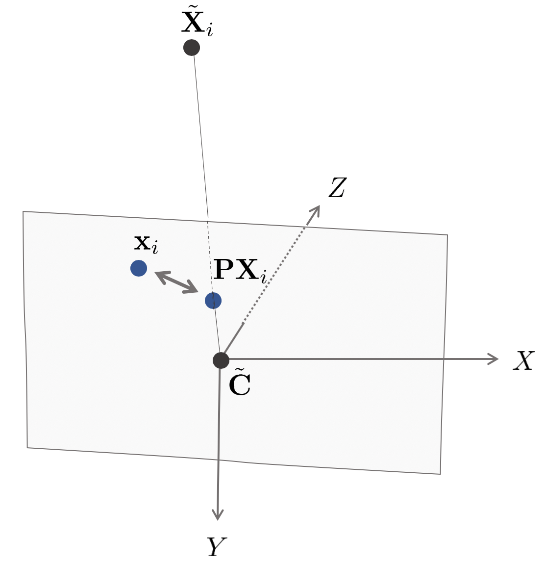
2.1.1. The basic pinhole model
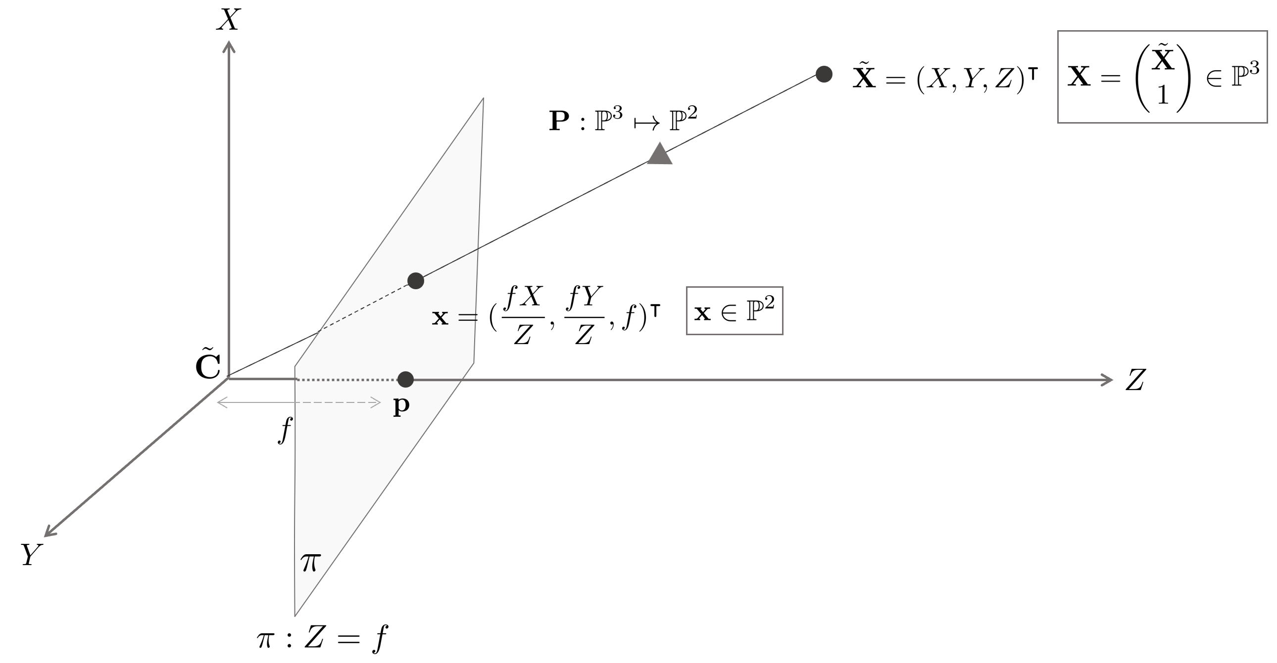
핀홀 카메라(pinhole camera)란 $\mathbb{R}^{3}$ 공간 상에 있는 한 점 $\tilde{\mathbf{X}}$를 특정 중심점 $\tilde{\mathbf{C}}$를 향해 프로젝션시켰을 때 중간에 교차하는 이미지 평면 $\pi \in \mathbb{R}^{2}$ 상의 한 점 $\mathbf{x}$으로 상을 맺음으로써 이미지를 표현하는 수학적인 카메라 모델링 방법을 의미한다. $\tilde{\mathbf{X}}, \tilde{\mathbf{C}}$는 Inhomogeneous Coordinate으로 나타낸 $\mathbf{X}$를 의미한다.
\begin{equation}
\begin{aligned}
& \mathbf{X} = \begin{bmatrix} X&Y&Z&1 \end{bmatrix}^{\intercal} \\
& \tilde{\mathbf{X}} = \begin{bmatrix} X&Y&Z \end{bmatrix}^{\intercal} \\
& \mathbf{C} = \begin{bmatrix} c_{x}&c_{y}&c_{z}&1 \end{bmatrix}^{\intercal} \\
& \tilde{\mathbf{C}} = \begin{bmatrix} c_{x}&c_{y}&c_{z}\end{bmatrix}^{\intercal} \\
\end{aligned}
\end{equation}
임의의 $\mathbb{R}^{3}$ 공간을 카메라 좌표계라고 생각해보면 좌표계의 원점은 카메라의 중심점 $\tilde{\mathbf{C}}$가 된다. 일반적으로 이미지 평면 $\pi$은 $Z$축과 수직하도록 위치시키며 이 때, $Z$축을 Principal Axis라고 하고 이미지 평면과 Principal Axis가 만나는 점을 Principal Point $\mathbf{p}$라고 한다.
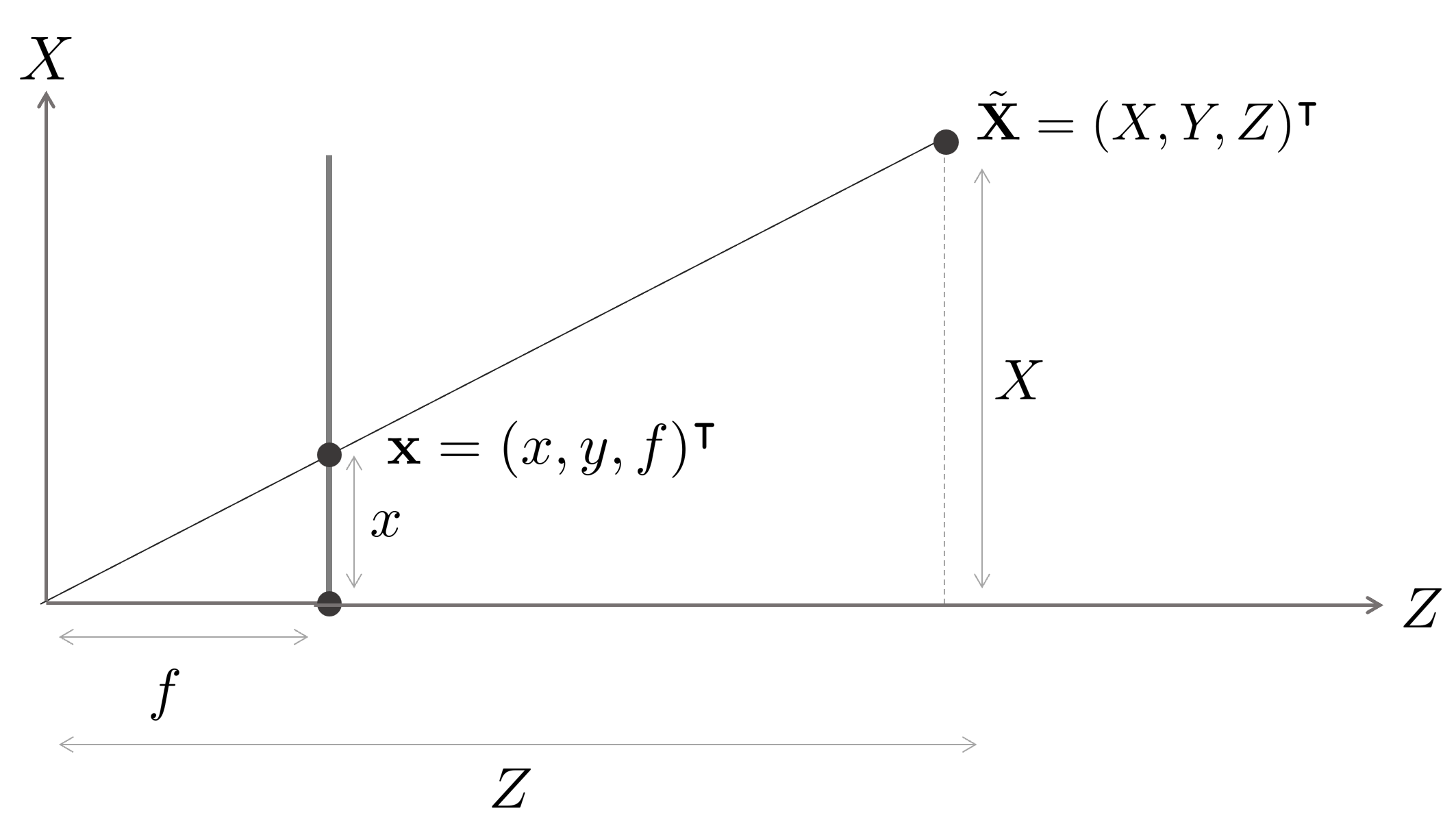
3차원 공간 상의 점 $\tilde{\mathbf{X}} = \begin{bmatrix} X&Y&Z \end{bmatrix}^{\intercal}$가 주어졌을 때 $XZ$ 평면만 보는 경우 이미지 평면 $\pi$과 카메라 중심점 $\tilde{\mathbf{C}}$ 사이의 거리인 $X$축에 대한 초점거리(focal length) $f_{x}$를 계산할 수 있다. $f_x, f_y$는 픽셀의 종횡비를 의미하지만 최근 생산되는 센서는 대부분 종횡비가 1:1이므로 $f=f_{x}=f_{y}$라고 가정한다.
\begin{equation}
\begin{aligned}
f\frac{Y}{Z} = y
\end{aligned}
\end{equation}
$YZ$ 평면에서 이미지 평면을 봤을 때 역시 동일하게 $f$를 계산할 수 있다.
\begin{equation}
\begin{aligned}
f\frac{X}{Z} = x
\end{aligned}
\end{equation}
이에 따라 핀홀 카메라 행렬 $\mathbf{P}$는 월드 상의 점 $\tilde{\mathbf{X}} = \begin{pmatrix} X&Y&Z \end{pmatrix}^{\intercal} \in \mathbb{R}^{3}$를 2차원 이미지 평면 $\pi \in \mathbb{R}^{2}$로 프로젝션하는 선형 사상이라고 볼 수 있다.
\begin{equation}
\begin{aligned}
\mathbf{P}: (X,\ Y,\ Z)^{\intercal} \ \mapsto \ (f \frac{X}{Z},\ f\frac{Y}{Z})^{\intercal}
\end{aligned}
\end{equation}
2.1.2. Central projection using homogeneous coordinates
핀홀 카메라 행렬 $\mathbf{P}$은 Homogeneous Point를 옮기는 것으로 생각할 수도 있다. 다시 말하면, 핀홀 카메라 행렬 $\mathbf{P}$는 $\mathbb{P}^{3}$ 공간 상의 점 $\mathbf{X}=\begin{pmatrix} X&Y&Z&1 \end{pmatrix}^{\intercal}$을 $\mathbb{P}^{2}$ 공간 상의 점 $\mathbf{x}=\begin{pmatrix} fX&fY&Z \end{pmatrix}^{\intercal}$로 프로젝션하는 선형 사상으로 볼 수 있다.
\begin{equation}
\begin{aligned}
\mathbf{P}: \begin{pmatrix} X\\Y\\Z\\1 \end{pmatrix} \mapsto \begin{pmatrix} fX \\ fY \\ Z \end{pmatrix} = \begin{bmatrix} f&&&0 \\ &f&&0 \\ &&1&0 \end{bmatrix}\begin{pmatrix} X\\Y\\Z\\1 \end{pmatrix}
\end{aligned}
\end{equation}
이를 행렬 형태로 나타내면
\begin{equation}
\begin{aligned}
\mathbf{x} = \mathbf{PX}
\end{aligned}
\end{equation}
가 된다. 이 때, $\mathbf{P} = \text{diag}(f,f,1)[\mathbf{I}\ |\ 0 ]_{3\times4}$와 같이 나타낼 수 있다.
2.1.3. Principal point offset
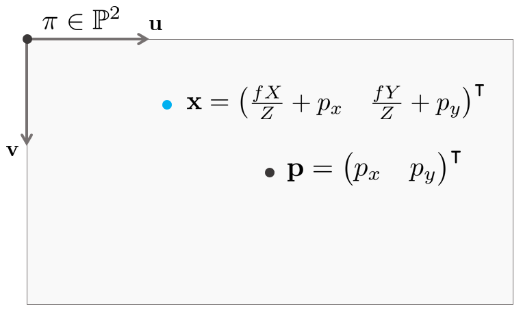
일반적으로 Principal Point $\mathbf{p}$는 이미지 평면 $\pi$의 원점이 아니다. 따라서 핀홀 카메라 행렬을 통한 선형 사상이 이미지 평면 $\pi$에 제대로 대응하기 위해서는
\begin{equation}
\begin{aligned}
\begin{pmatrix} X&Y&Z \end{pmatrix}^{\intercal} \mapsto \begin{pmatrix} fX/Z + p_{x} & fY/Z+p_{y} \end{pmatrix}^{\intercal}
\end{aligned}
\end{equation}
와 같이 Printcipal Point $\mathbf{p}=\begin{pmatrix} p_{x} & p_{y} \end{pmatrix}^{\intercal}$를 보정해야 한다. 이를 카메라 행렬 $\mathbf{P}$를 통해 한 번에 표현해보면
\begin{equation}
\begin{aligned}
\mathbf{P}: \begin{pmatrix} X\\Y\\Z\\1 \end{pmatrix} \mapsto \begin{pmatrix} fX+Zp_{x} \\ fY+Zp_{y} \\ Z \end{pmatrix} = \begin{bmatrix} f&&p_{x}&0 \\ &f&p_{y}&0 \\ &&1&0 \end{bmatrix}\begin{pmatrix} X\\Y\\Z\\1 \end{pmatrix}
\end{aligned}
\end{equation}
와 같이 나타낼 수 있다. 이 때 행렬 $\begin{bmatrix} f&&p_{x} \\ &f&p_{y} \\ &&1 \end{bmatrix}$을 간결하게 $\mathbf{K}$로 나타내며 이를 내부 파라미터 또는 카메라 캘리브레이션 행렬(intrinsic parameter matrix, camera calibration matrix)이라고 한다.
\begin{equation}
\begin{aligned}
\mathbf{K} = \begin{bmatrix} f&&p_{x} \\ &f&p_{y} \\ &&1 \end{bmatrix}
\end{aligned}
\end{equation}
결론적으로 카메라의 Principal Point Offset을 포함한 카메라 행렬 $\mathbf{P}$를 통해 다음과 같은 $\mathbf{X} \in \mathbb{P}^{3} \mapsto \mathbf{x} \in \mathbb{P}^{2}$인 선형 사상이 가능하다.
\begin{equation}
\begin{aligned}
\mathbf{x} = \mathbf{K}[\mathbf{I}\ | \ 0]\mathbf{X}
\end{aligned}
\end{equation}
2.1.4. Camera rotation and translation
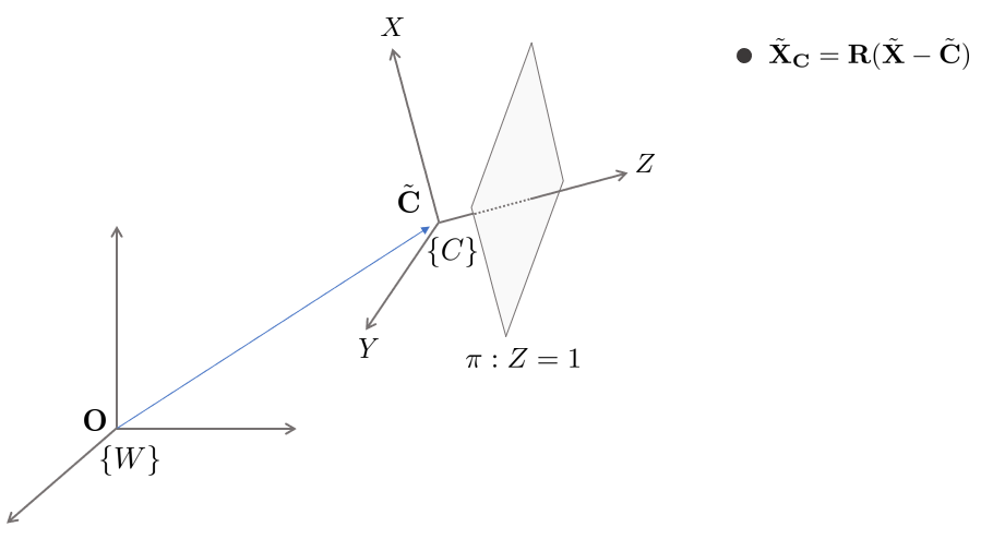
일반적으로 카메라 좌표계는 월드 좌표계와 동일하지 않다. $\mathbb{R}^{3}$ 공간 상에 월드 좌표계 $\{W\}$가 주어졌을 때 이로부터 위치가 $\mathbf{C}=\begin{pmatrix} c_{x}&c_{y}&c_{z}&1 \end{pmatrix}^{\intercal}$만큼 떨어져 있으며 $\mathbf{R}$만큼 회전되어 있는 카메라 좌표계 $\{C\}$가 주어졌을 때 월드 좌표계 $\{W\}$에서 바라본 월드 상의 한 점 $\tilde{\mathbf{X}}$를 카메라 좌표계 $\{C\}$ 상의 점 $\tilde{\mathbf{X}}_{\mathbf{C}}$로 변환하는 공식은
\begin{equation}
\begin{aligned}
\tilde{\mathbf{X}}_{\mathbf{C}} = \mathbf{R}(\tilde{\mathbf{X}}-\tilde{\mathbf{C}})
\end{aligned}
\end{equation}
와 같다. Homogeneous Coordinate로 나타낸 $\mathbf{X}_{\mathbf{C}}$를 이미지 평면 $\pi$로 프로젝션시키면
\begin{equation}
\begin{aligned}
\mathbf{x} = \mathbf{P}\mathbf{X}_{\mathbf{C}} = \mathbf{K}[\mathbf{I}\ | \ 0]\mathbf{X}_{\mathbf{C}}
\end{aligned}
\end{equation}
와 같이 나타낼 수 있다. $\mathbf{X}_{\mathbf{C}}$를 자세히 나타내면
\begin{equation}
\begin{aligned}
\mathbf{X}_{\mathbf{C}} & = \mathbf{R} \begin{bmatrix} 1&&&-c_{x} \\&1&&-c_{y} \\ &&1&-c_{z} \end{bmatrix} \begin{bmatrix} X\\Y\\Z\\1 \end{bmatrix} \\
& = \begin{bmatrix} \mathbf{R} & -\mathbf{R}\tilde{\mathbf{C}} \\ 0 & 1 \end{bmatrix}\begin{bmatrix} X\\Y\\Z\\1 \end{bmatrix} \quad \text{in homogenous coord}
\end{aligned}
\end{equation}
과 같이 나타낼 수 있고 이를 $\mathbf{x} = \mathbf{K}[\mathbf{I}\ | \ 0]\mathbf{X}_{\mathbf{C}}$ 공식에 대입 후 정리하면
\begin{equation}
\begin{aligned}
\mathbf{x} & = \mathbf{K} [\mathbf{I} \ | \ 0 ]\mathbf{X}_{\mathbf{C}}\\
& = \mathbf{K}[\mathbf{I} \ | \ 0]\begin{bmatrix} \mathbf{R} & -\mathbf{R}\tilde{\mathbf{C}} \\ 0 & 1 \end{bmatrix}\begin{bmatrix} X\\Y\\Z\\1 \end{bmatrix} \\
& = \mathbf{K} [\mathbf{R} \ | \ -\mathbf{R}\tilde{\mathbf{C}}]\mathbf{X} \\
& = \mathbf{KR}[\mathbf{I} \ | \ -\tilde{\mathbf{C}}]\mathbf{X}
\end{aligned}
\end{equation}
와 같이 나타낼 수 있다. 일반적으로 $\tilde{\mathbf{X}}_{\mathbf{C}}$를 $\tilde{\mathbf{X}}_{\mathbf{C}}=\mathbf{R}\tilde{\mathbf{X}} + \mathbf{t}$와 같이 월드 좌표계를 기준으로 표현하는 방법 또한 자주 사용된다. 이 때 카메라 행렬 $\mathbf{P}$는
\begin{equation}
\begin{aligned}
\mathbf{P} = \mathbf{K}[\mathbf{R} \ | \ \mathbf{t}]
\end{aligned}
\end{equation}
와 같이 나타낼 수 있고 이 때, $\mathbf{t} = -\mathbf{R}\tilde{\mathbf{C}}$ 관계가 성립한다.
2.1.5. CCD cameras
현대에 주로 사용하는 카메라 중 하나인 CCD 카메라는 이미지 좌표를 픽셀의 수로 기록한다. 따라서 $(x,y) [mm]$와 같이 이미지 좌표가 mm로 주어져 있을 때, CCD 카메라에서는 $(m_{x}x,\ m_{y}y)$와 같이 나타낸다. 이 때 $m_{x}, m_{y}$는 1 $mm^{2}$ 크기 내에서 x축 또는 y축 방향으로 픽셀의 수를 의미한다. 따라서 mm로 주어진 일반 카메라 캘리브레이션 행렬 $\mathbf{K}$가 주어졌을 때 이를 CCD 카메라의 좌표계로 바꾸기 위해서는
\begin{equation}
\begin{aligned}
\begin{pmatrix} m_{x}&& \\ &m_{y}& \\ &&1 \end{pmatrix} \mathbf{K} = \begin{pmatrix} m_{x}&& \\ &m_{y}& \\ &&1 \end{pmatrix} \begin{pmatrix} f&&p_{x} \\ &f&p_{y} \\ && 1 \end{pmatrix} = \begin{pmatrix} fm_{x} && p_{x}m_{x} \\ &fm_{y} & p_{y}m_{y} \\ 0&0&1 \end{pmatrix}
\end{aligned}
\end{equation}
와 같이 변환하는 작업을 수행해야 한다.
2.1.6. Finite projective camera
카메라 행렬이 $\mathbf{P}=\mathbf{K}[\mathbf{R} \ | \ \mathbf{t}]$와 같이 주어졌을 때 이를 다시 표현하면
\begin{equation}
\begin{aligned}
\mathbf{P} = \mathbf{KR} [ \mathbf{I} \ | \ -\tilde{\mathbf{C}}] \quad \text{where, } \mathbf{t} = -\mathbf{R}\tilde{\mathbf{C}}
\end{aligned}
\end{equation}
과 같이 나타낼 수 있고 해당 카메라 행렬을 Finite Projective 카메라라고 하며 이 때 $\mathbf{KR}$가 non-singular한 행렬이 되어야 한다. 임의의 non-singular 행렬 $\mathbf{M} \in \mathbb{R}^{3\times 3}$가 주어졌을 때 $\mathbf{M}$에 QR factorization을 수행하는 $\mathbf{KR}$과 같이 상삼각행렬 $\mathbf{K}$와 직교행렬 $\mathbf{R}$로 분해할 수 있으므로 따라서 카메라 행렬의 집합은 $\mathbf{P} \in \mathbb{R}^{3\times 4}$ 크기의 행렬들의 집합이고 $\mathbf{P}$의 왼쪽 $3\times3$ 부분이 non-singular인 집합이다.
\begin{equation}
\begin{aligned}
\{\text{set of camera matrix}\} = \{ \mathbf{P} = [\mathbf{M} \ | \ \mathbf{t}] \ | \ \mathbf{M} \text{ is non-singular } 3\times 3 \text{ matrix.}, \mathbf{t} \in \mathbb{R}^{3} \}
\end{aligned}
\end{equation}
2.1.7. General projective cameras
General Projective Camera는 앞서 설명한 Finite projective camera와 달리 $\mathbf{P} = [\mathbf{M} \ | \ \mathbf{t}]$에서 $\mathbf{M} \in \mathbb{R}^{3\times 3}$ 행렬이 non-singular일 필요가 없으며 $\mathbf{P}$의 rank가 3인 카메라 행렬을 의미한다.
2.2. The projective camera
2.2.1. Camera anatomy
2.2.2. Camera center
임의의 Finite Projective 카메라 행렬 $\mathbf{P} = \mathbf{KR}[\mathbf{I} \ | \ -\tilde{\mathbf{C}}]$가 주어졌을 때
\begin{equation}
\begin{aligned}
\mathbf{PC} = \mathbf{KR}(\mathbf{C}-\mathbf{C}) = \mathbf{0}
\end{aligned}
\end{equation}
이 된다. 이 때, $\mathbf{C} \in \mathbb{R}^{4}$는 카메라의 중심점 또는 월드 좌표계 상에서 카메라의 위치를 의미하고 rank 3인 카메라 행렬 $\mathbf{P} \in \mathbb{R}^{3\times 4}$의 Null Space 벡터를 구함으로써 카메라 중심점을 구할 수 있다.
카메라 행렬 $\mathbf{P}=\mathbf{KR}[\mathbf{I} \ | \ -\tilde{\mathbf{C}}]$가 주어졌고 $\mathbf{PC} = \mathbf{0}$이 성립할 때 다음과 같이 월드 상의 점 $\mathbf{X}(\lambda)$가 주어졌다고 하자.
\begin{equation}
\begin{aligned}
\mathbf{X}(\lambda) = \lambda\mathbf{A} + (1-\lambda)\mathbf{C}
\end{aligned}
\end{equation}
이는 곧 $\mathbf{A}$와 $\mathbf{C}$를 잇는 직선을 의미하며 $\mathbf{X}(\lambda)$를 카메라에 프로젝션시키면
\begin{equation}
\begin{aligned}
\mathbf{x} = \mathbf{PX}(\lambda) = \lambda\mathbf{P}\mathbf{A} + (1-\lambda)\mathbf{PC} = \lambda \mathbf{PA}
\end{aligned}
\end{equation}
가 된다. 즉, 월드 상의 점 $\mathbf{A}$와 $\mathbf{C}$를 잇는 직선이 $\mathbf{C}$ 값에 관계없이 이미지 평면 상의 한 점 $\mathbf{x}=\mathbf{\lambda}\mathbf{PA}$가 된다는 의미이고 이는 곧 카메라의 중심점이 가지는 성질을 의미한다. 일반적인 General Projective Camera에서도 $\mathbf{P}$의 Null Space 벡터가 곧 카메라의 중심점 $\mathbf{C}$가 된다.
2.2.3. Column vectors
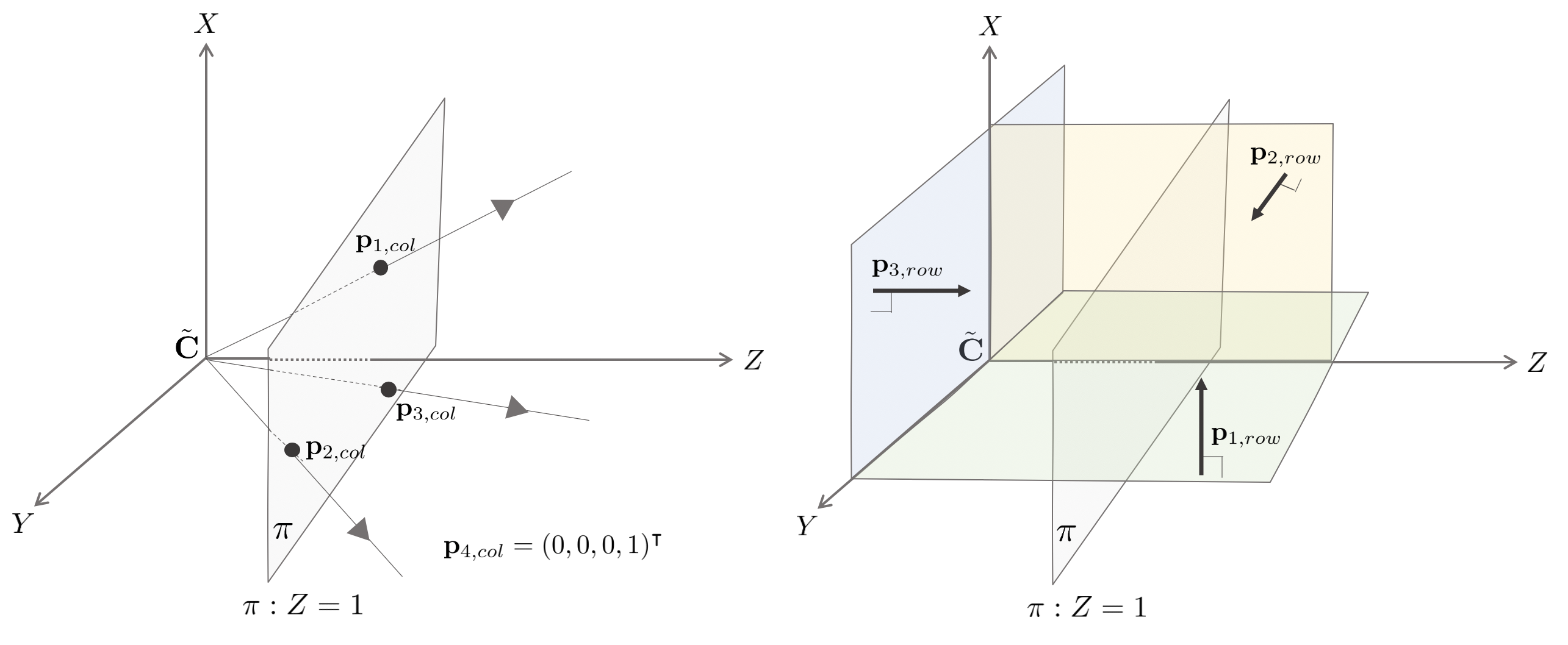
카메라 행렬 $\mathbf{P}$을 열벡터(column vector)로 나타내면 다음과 같다.
\begin{equation}
\begin{aligned}
& \mathbf{P} = \begin{bmatrix} \mathbf{p}_{1,col} & \mathbf{p}_{2,col} & \mathbf{p}_{3,col} & \mathbf{p}_{4,col} \end{bmatrix}\\
& \text{where, } \mathbf{p}_{i,col} \in \mathbb{R}^{3\times1}, \ i=1,\cdots,4
\end{aligned}
\end{equation}
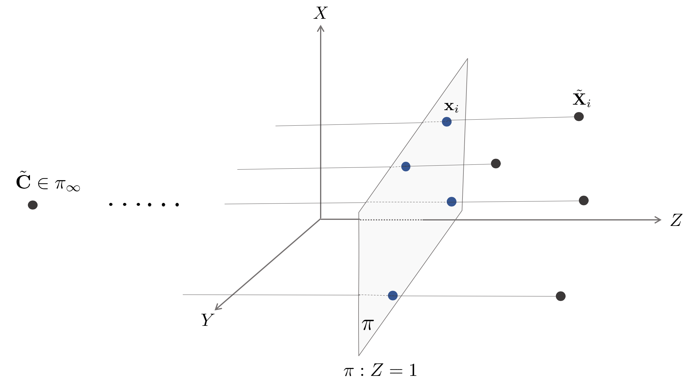
이 중 $\mathbf{p}_{i,col}, \ i=1,2,3$은 각각 무한대 평면 $\pi_{\infty}$에 위치한 $X,Y,Z$축의 소실점(vanisinh point)들의 위치를 의미한다. 그리고 $\mathbf{p}_{4,col} = \mathbf{P} \begin{pmatrix} 0&0&0&1 \end{pmatrix}^{\intercal}$은 윌드 좌표계의 원점을 의미한다.
2.2.4. Row vectors
카메라 행렬 $\mathbf{P}$을 행벡터(row vector)로 나타내면 다음과 같다.
\begin{equation}
\begin{aligned}
& \mathbf{P} = \begin{bmatrix} \mathbf{p}_{1,row}^{\intercal} \\ \mathbf{p}_{2,row}^{\intercal} \\ \mathbf{p}_{3,row}^{\intercal} \end{bmatrix}\\
& \text{where, } \mathbf{p}_{i,row} \in \mathbb{R}^{4\times1}, \ i=1,2,3
\end{aligned}
\end{equation}
행벡터 $\mathbf{p}_{i,row}, \ i=1,2,3$은 카메라 좌표계 기준으로 각각 $X,Y,Z$ 축과 평행한 평면을 의미한다.
2.2.5. The principal plane
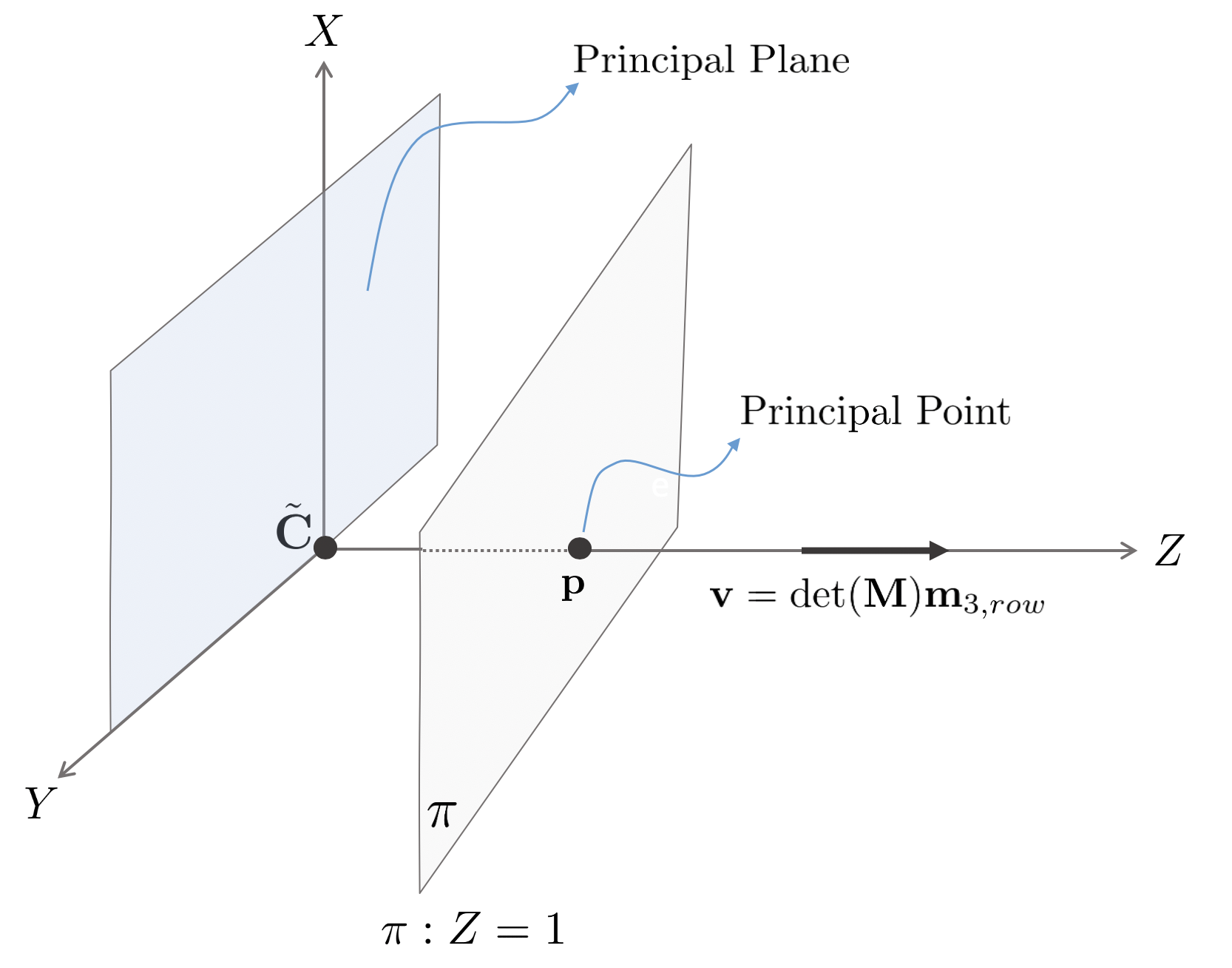
주평면(principal plane) $\pi_{pp}$은 카메라의 중심점(center)를 포함하며 이미지 평면과 평행인 평면을 의미한다. 주평면은 카메라 좌표계 $\{C\}$에서 $XY$ 평면과 동일하며 $Z=0$인 특징이 있다. 주평면 상에 위치하는 한 점 $\mathbf{X} \in \pi_{pp}$는 무한대 선(line at infinity) 상에서 이미지 평면 $\pi$과 만나므로
\begin{equation}
\begin{aligned}
\mathbf{x} = \mathbf{PX} = \begin{pmatrix} x&y&0 \end{pmatrix}^{\intercal}
\end{aligned}
\end{equation}
이 되고 따라서 임의의 한 점 $\mathbf{X}$가 주평면 상에 위치하기 위한 필요충분 조건은 $\mathbf{p}_{3,row}^{\intercal}\mathbf{X} = 0$이다. 즉, 카메라 행렬의 세 번째 행벡터 $\mathbf{p}_{3,row}$가 곧 카메라의 주평면을 의미한다.
2.2.6. The principal point
주점(principal point) $\mathbf{p}$는 주축(principal axis)와 이미지 평면 $\pi$의 교차점을 의미한다. 주점 $\mathbf{p}$는 이미지 평면 $\pi$ 상에 위치하며 카메라 중심점 $\mathbf{C}$와 주점을 잇는 직선은 이미지 평면과 수직하다.
\begin{equation}
\begin{aligned}
\mathbf{p}-\mathbf{C} \perp \pi
\end{aligned}
\end{equation}
다음과 같은 방법으로 주점을 정의할 수도 있다. 주평면은 카메라 행렬의 세 번째 행벡터 $\mathbf{p}_{3,row}$이므로 주평면 상에 위치한 한 점 $\mathbf{X}$에 대해
\begin{equation}
\begin{aligned}
\mathbf{p}_{3,row}^{\intercal}\mathbf{X} = 0
\end{aligned}
\end{equation}
이 성립한다. 이 때 $\mathbf{p}_{3,row} = \begin{pmatrix} \pi_{1}&\pi_{2}&\pi_{3}&\pi_{4} \end{pmatrix}^{\intercal}$는 Dual Projective Space $(\mathbb{P}^{3})^{\vee}$에서 $\mathbf{p}_{3,row}$ 평면의 법선벡터를 의미한다. 주평면 $\mathbf{p}_{3,row}$와 무한대 평면(plane at infinity) $\pi_{\infty}$의 교차선은 무한대 평면에 존재하는 법선벡터 $\begin{pmatrix} \pi_{1}&\pi_{2}&\pi_{3}&0 \end{pmatrix}^{\intercal}$가 된다. 결론적으로 이를 이미지 평면으로 프로젝션한 점이 주점(principal point) $\mathbf{p}$가 된다.
\begin{equation}
\begin{aligned}
\mathbf{p} = \mathbf{P} \begin{pmatrix} \pi_{1}\\\pi_{2}\\\pi_{3}\\0 \end{pmatrix}
\end{aligned}
\end{equation}
카메라 중심점 $\mathbf{C}$를 지나면서 무한대 평면 상에 존재하는 법선벡터 $\begin{bmatrix} \pi_{1}&\pi_{2}&\pi_{3}&0 \end{bmatrix}^{\intercal}$는 곧 주축(principal axis)와 동일하므로
\begin{equation}
\begin{aligned}
\mathbf{P}\bigg( \lambda \begin{pmatrix} \pi_{1}\\\pi_{2}\\\pi_{3}\\0 \end{pmatrix} + (1-\lambda)\mathbf{C} \bigg) = \lambda \mathbf{P}\begin{pmatrix} \pi_{1}\\\pi_{2}\\\pi_{3}\\0 \end{pmatrix} = \mathbf{p}
\end{aligned}
\end{equation}
같이 주축을 이미지 평면에 프로젝션하면 주점 $\mathbf{p}$이 된다. 결론적으로 주점 $\mathbf{p}$는 카메라 행렬 $\mathbf{P}$의 세번째 행벡터 $\mathbf{p}_{3,row} = \begin{bmatrix} \pi_{1}&\pi_{2}&\pi_{3}&p_{4} \end{bmatrix}^{\intercal}$에서 처음 세 개의 항 $\mathbf{p} = (\pi_{1},\pi_{2},\pi_{3})^{\intercal}$을 의미한다.
2.2.7. The principal axis vector
카메라 행렬 $\mathbf{P} = [\mathbf{M} \ | \ \mathbf{p}_{4,col}]$이 주어졌을 때 행렬 $\mathbf{M} \in \mathbb{R}^{3\times 3}$의 세 번째 행벡터 $\mathbf{m}_{3,row}$는 주점(principal point)를 의미한다. 해당 섹션에서는 주점 $\mathbf{m}_{3,row}$를 카메라 좌표계에서 $+Z$ 방향을 의미하는 주축(principal axis)의 방향과 동치로 간주한다. 하지만, 카메라 행렬 $\mathbf{P}$는 부호를 제외하고(up to sign) 유일하게 결정되기 때문에 어떤 $\mathbf{m}_{3,row}$ 또는 $-\mathbf{m}_{3,row}$가 $+Z$를 의미하는지 알 수 없다.
이 때, $\mathbf{v} = \det(\mathbf{M})\mathbf{m}_{3,row} = (0,0,1)^{\intercal}$과 같이 $\mathbf{M}$의 행렬식(determinant)를 앞에 곱해주면 항상 양의 방향을 의미하게 된다. 그리고 $\mathbf{P} \rightarrow k \mathbf{P}$로 스케일이 변화해도 $\mathbf{v} \rightarrow k^{4}\mathbf{v}$와 같이 같은 방향을 나타낸다. 일반적인 카메라 행렬 $k\mathbf{P} = k\mathbf{KR}[\mathbf{I} \ | \ -\tilde{\mathbf{C}}]$가 주어졌을 때에도 $\mathbf{M} = k \mathbf{KR}$이고 $\det(\mathbf{R}) > 0$이므로 주축의 방향벡터 $\mathbf{v}=\det(\mathbf{M})\mathbf{m}_{3,rowe}$는 동일한 방향을 나타낸다. 이에 따라
\begin{equation}
\begin{aligned}
\mathbf{v} = \det(\mathbf{M})\mathbf{m}_{3,row}
\end{aligned}
\end{equation}
벡터는 주축(principal axis)의 방향벡터를 의미한다.
2.2.8. Action of a projective camera on points
2.2.9. Forward projection
Forward-projection은 일반적으로 프로젝션이라고 불리며 월드 상에 있는 한 점 $\mathbf{X}$가 주어졌을 때 이를 이미지 평면 상의 한 점 $\mathbf{x}$으로 변환하는 연산을 의미한다. 임의의 카메라 행렬 $\mathbf{P}$에 대해 다음 공식이 성립한다.
\begin{equation}
\begin{aligned}
\mathbf{x} = \mathbf{PX}
\end{aligned}
\end{equation}
2.2.10. Back-projection of points to rays
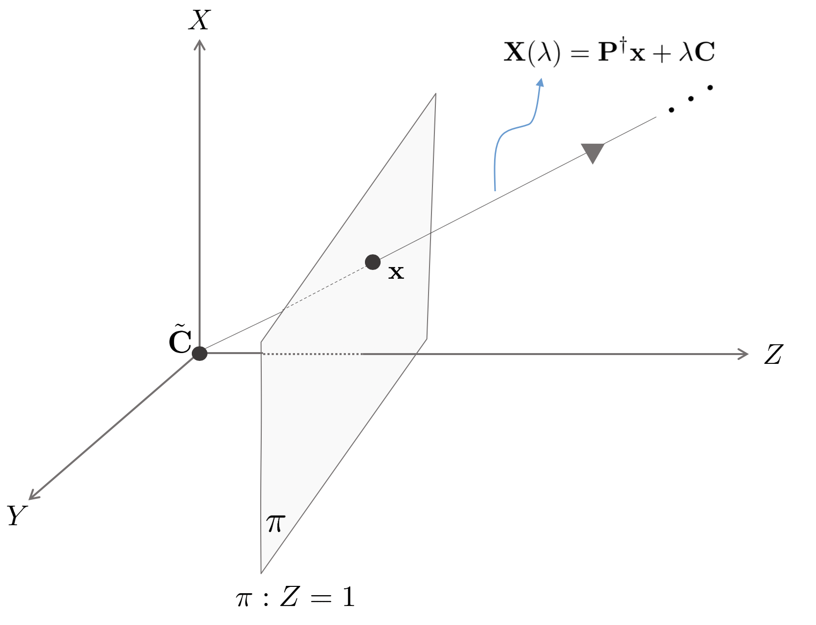
Back-projection은 Forward-projection과는 반대로 이미지 평면 상의 한 점 $\mathbf{x}$가 주어졌을 때 이를 월드 상의 한 직선으로 변환하는 연산을 의미한다. 일반적으로 $\mathbf{x}$의 깊이값을 모르기 때문에 바로 월드 상의 한 점 $\mathbf{X}$로 변환되지 않는 특징이 있다. 임의의 카메라 행렬 $\mathbf{P}$는 rank가 3인 행렬이므로 Right Pseudo Inverse $\mathbf{P}^{\dagger}$가 존재한다.
\begin{equation}
\begin{aligned}
\mathbf{P}^{\dagger} = \mathbf{P}^{\intercal}(\mathbf{PP}^{\intercal})^{-1}
\end{aligned}
\end{equation}
이 때 $\mathbf{PP}^{\dagger} = \mathbf{PP}^{\intercal}(\mathbf{PP}^{\intercal})^{-1} = \mathbf{I}$가 성립한다. Back-projection한 직선 $\mathbf{P}^{\dagger}\mathbf{x}$는 카메라의 중심점 $\mathbf{C}$를 지나가므로
\begin{equation}
\begin{aligned}
\mathbf{X}(\lambda) = \mathbf{P}^{\dagger}\mathbf{x} + \lambda \mathbf{C}
\end{aligned}
\end{equation}
와 같이 나타낼 수 있다. Back-projection 직선을 다시 프로젝션하면 $\mathbf{P}\mathbf{X}(\lambda) = \mathbf{PP}^{\dagger}\mathbf{x} + \lambda \mathbf{PC} = \mathbf{x}$가 된다.
Finite Projective 카메라의 경우 다른 방법으로 Back-projection을 표현할 수 있다. 임의의 Finite Projective 카메라 행렬 $\mathbf{P}=[\mathbf{M} \ | \ \mathbf{p}_{4,col}]$이 주어졌을 때 카메라의 중심점은 $\tilde{\mathbf{C}}=-\mathbf{M}^{-1}\mathbf{p}_{4,col}$과 같이 나타낼 수 있다. 이 때 이미지 평면 상의 한 점 $\mathbf{x}$을 Back-projection한 직선은 무한대 평면 $\pi_{\infty}$와 $\mathbf{D}=((\mathbf{M}^{-1}\mathbf{x})^{\intercal},0)$에서 접하므로 Back-projection 직선은
\begin{equation}
\begin{aligned}
\mathbf{X}(\mu) = \mu \begin{pmatrix} \mathbf{M}^{-1}\mathbf{x}\\0 \end{pmatrix} + \begin{pmatrix} -\mathbf{M}^{-1}\mathbf{p}_{4,col} \\ 1 \end{pmatrix} = \begin{pmatrix} \mathbf{M}^{-1}(\mu \mathbf{x} - \mathbf{p}_{4,col}) \\ 1 \end{pmatrix}
\end{aligned}
\end{equation}
과 같이 나타낼 수 있다.
2.2.11. Depth of points
General Projective 카메라 $\mathbf{P}$와 월드 상의 한 점 $\mathbf{X}=\begin{pmatrix} X&Y&Z&1 \end{pmatrix}^{\intercal}$가 주어졌을 때 이를 이미지 평면으로 프로젝션시키면
\begin{equation}
\begin{aligned}
\mathbf{x} = \mathbf{P}\begin{pmatrix} X\\Y\\Z\\1 \end{pmatrix} = \begin{pmatrix} x\\y\\w \end{pmatrix}
\end{aligned}
\end{equation}
와 같이 하나의 점 $\mathbf{x}$를 얻을 수 있다.
2.2.12. Result 6.1
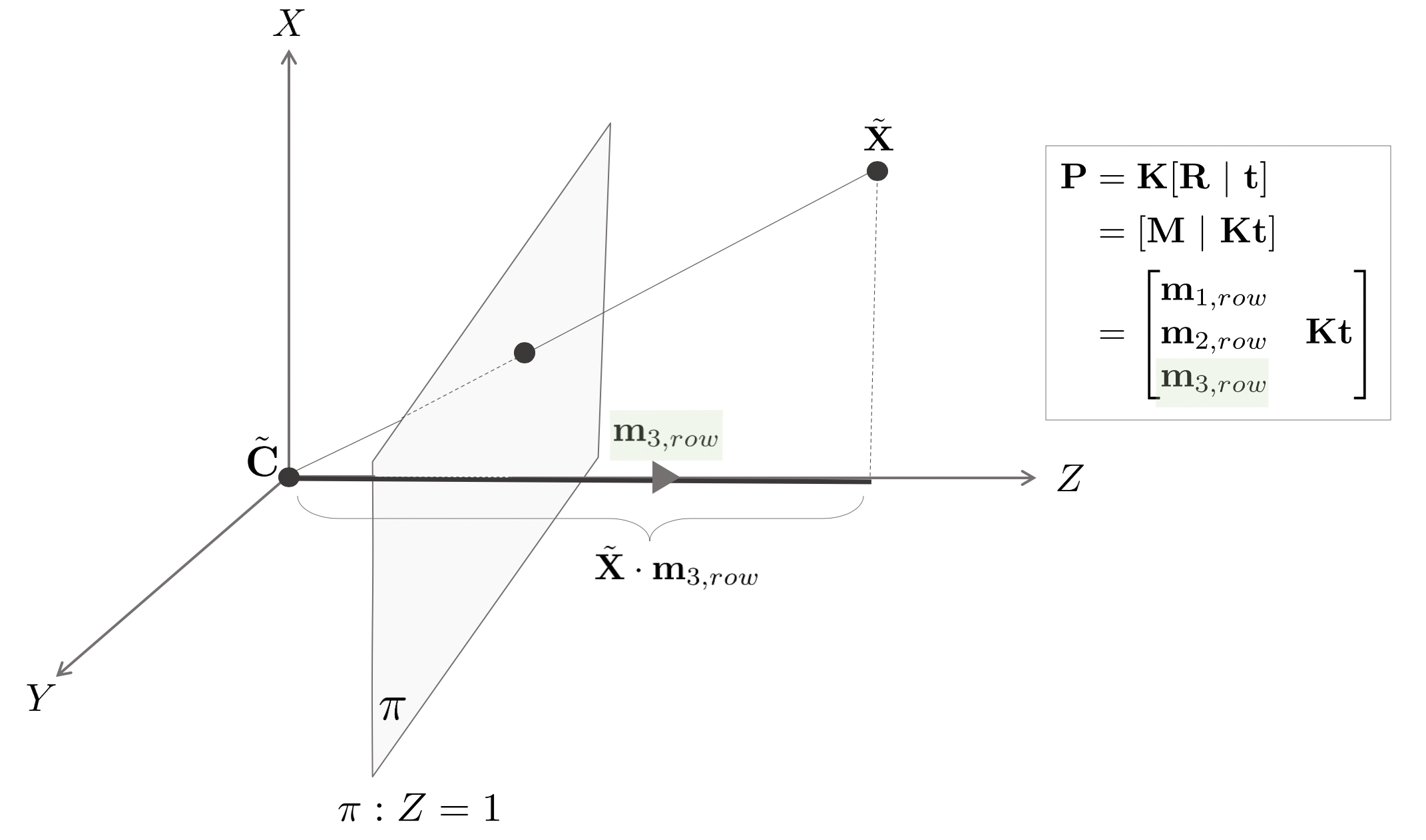
카메라 행렬 $\mathbf{P}$에 대한 월드 상의 점 $\mathbf{X}$의 깊이는
\begin{equation}
\begin{aligned}
\text{depth}(\mathbf{X}; \mathbf{P}) = \frac{\text{sign}(\det(M))w}{\|\mathbf{m}_{3,row} \|}
\end{aligned}
\end{equation}
와 같이 나타낼 수 있다. 이 때, $\mathbf{m}_{3,row} \in \mathbb{R}^{3\times 3}$는 행렬 $\mathbf{M}$의 세번째 행벡터이다.
2.2.13. Proof
행벡터 $\mathbf{m}_{3,row}$는 주축의 방향을 의미하므로 월드 상의 점 $\tilde{\mathbf{X}}$를 $\mathbf{m}_{3,row}$로 프로젝션한 값이 곧 $Z$축에 대한 깊이를 의미한다. 주축으로 프로젝션은
\begin{equation}
\begin{aligned}
\text{depth} = \frac{(\tilde{\mathbf{X}}-\tilde{\mathbf{C})}\mathbf{m}_{3.row}}{\| \mathbf{m}_{3,row} \|}
\end{aligned}
\end{equation}
이 되고 Finite Projective 카메라의 경우 $\mathbf{m}_{3,row} = \mathbf{r}_{3,row} = 1$이 된다.
깊이 값은 $\mathbf{x} = \mathbf{PX}$의 세 번째 행인 $w$이므로
\begin{equation}
\begin{aligned}
w & = (\mathbf{PX})_{3,row} \\
& = (\mathbf{P}(\mathbf{X}-\mathbf{C}))_{3,row} \\
& = (\tilde{\mathbf{X}}-\tilde{\mathbf{C}})\mathbf{m}_{3,row} \\
\end{aligned}
\end{equation}
와 같이 구할 수 있다. 결론적으로 $\det(\mathbf{M})$의 부호에 따라 깊이 값이 카메라 뒤쪽에 위치할 수 있으므로 이를 고려하여 나타내면 다음과 같다.
\begin{equation}
\begin{aligned}
\text{depth}(\mathbf{X}; \mathbf{P}) = \frac{\text{sign}(\det(M))w}{\|\mathbf{m}_{3,row} \|}
\end{aligned}
\end{equation}
2.3. Cameras at infinity
임의의 General Projective 카메라의 중심점 $\mathbf{C}$가 무한대 평면 $\pi_{\infty}$에 존재하는 경우 이를 무한대 카메라(camera at infinity)라고 한다.
\begin{equation}
\begin{aligned}
\mathbf{C} =(\ast,\ \ast,\ \ast, 0)^{\intercal} \in \pi_{\infty}
\end{aligned}
\end{equation}
이와 동치(equivalent)인 경우는 카메라 행렬 $\mathbf{P}=[\mathbf{M} \ | \ \mathbf{p}_{4,col}]$가 주어졌을 때 행렬 $\mathbf{M}$가 singular한 경우이다.
무한대 카메라는 크게 Affine 카메라와 Non-affine 카메라로 분류된다.
2.3.1. Definition 6.3
Affine 카메라 $\mathbf{P}_{A}$는 무한대 평면을 프로젝션했을 때 동일하게 무한대 평면이 되는 카메라를 의미한다.
\begin{equation}
\begin{aligned}
\mathbf{P}_{A}(\pi_{\infty}) = \pi_\infty
\end{aligned}
\end{equation}
이 때, $\mathbf{P}_{A} = \begin{bmatrix} \ast&\ast&\ast&\ast \\ \ast&\ast&\ast&\ast \\ 0&0&0&\ast \end{bmatrix}$ 꼴이다.
2.3.2. Affine cameras
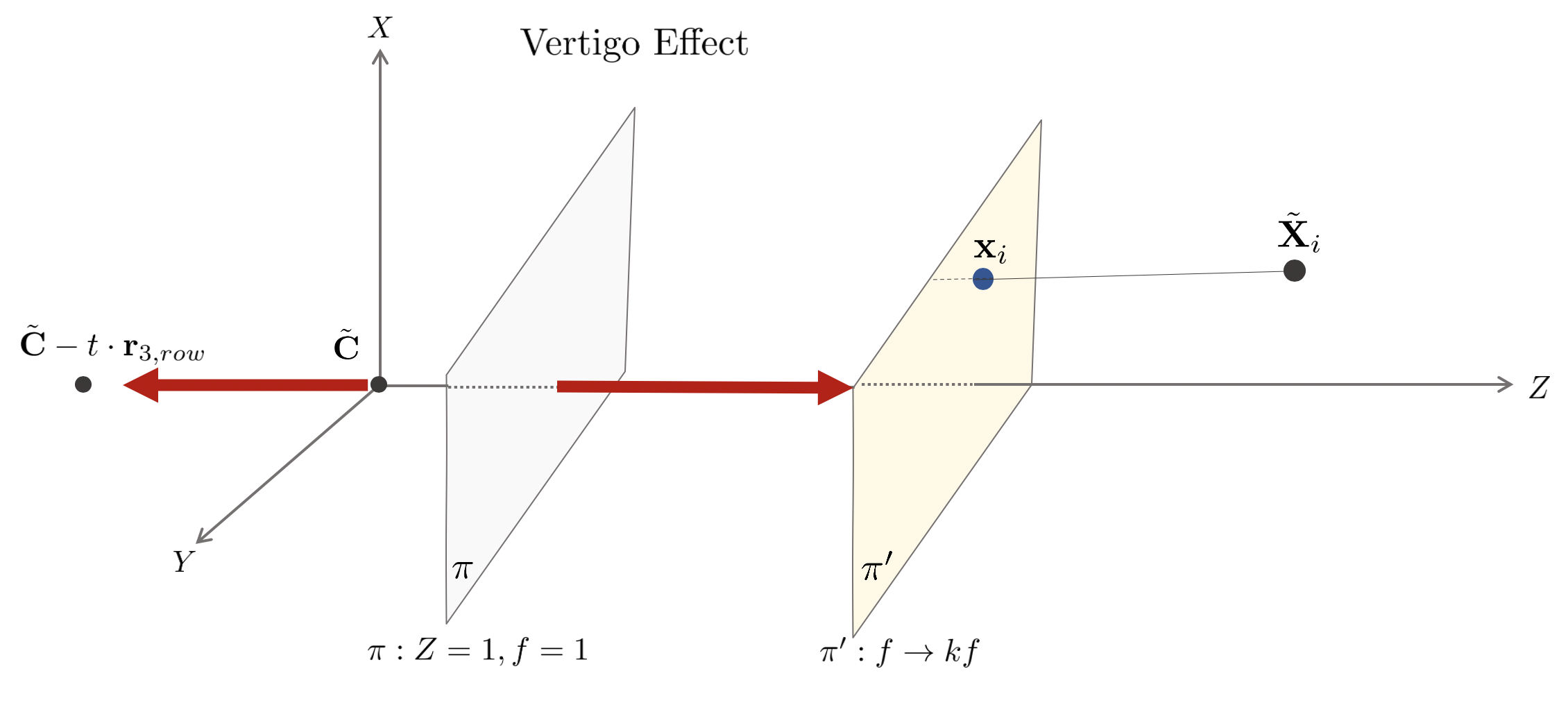
Finite Projective 카메라 행렬 $\mathbf{P}=\mathbf{KR}[\mathbf{I} \ | \ 0]$가 있고 월드 상의 물체가 존재한다고 하자. 이 때, 물체에 대한 Zoom In을 수행하면서 동시에 카메라를 주축의 반대 방향으로 움직이면 Vertigo Effect가 발생한다. Vertigo Effect는 히치콕 감독의 영화 Vertigo에서 해당 기법을 처음 사용해서 붙은 이름이다.
이를 수식적으로 이해하기 위해 월드 상 물체의 깊이(depth) 값에 대해 다시 생각해보면 카메라의 중심점 $\tilde{\mathbf{C}}$가 있고 월드 상의 점 $\tilde{\mathbf{X}}$가 주어졌을 때 깊이 값 $d$는
\begin{equation}
\begin{aligned}
d = -(\tilde{\mathbf{X}}-\tilde{\mathbf{C}})\mathbf{r}_{3,row}
\end{aligned}
\end{equation}
이다. 이 때, $\mathbf{r}_{3,row}$는 회전행렬 $\mathbf{R}$의 세 번째 행벡터이고 주축(principal axis)를 의미한다. 다음으로 카메라 중심점과 월드의 원점 사이의 거리를 $d_{0}$라고 하면 위 공식에서 $\tilde{\mathbf{X}}=0$인 경우에 해당하므로
\begin{equation}
\begin{aligned}
d_{0} = - \tilde{\mathbf{C}}\mathbf{r}_{3,row}
\end{aligned}
\end{equation}
이 된다.
카메라를 주축의 반대 방향으로 움직이면 카메라의 중심점 $\tilde{\mathbf{C}}$는
\begin{equation}
\begin{aligned}
\tilde{\mathbf{C}} - t\cdot \mathbf{r}_{3,row}
\end{aligned}
\end{equation}
이 되고 이 때, t는 시간을 의미한다. 카메라가 뒤로 움직일 때 시간에 따른 카메라 행렬은
\begin{equation}
\begin{aligned}
\mathbf{P}_{t} & = \mathbf{KR}[\mathbf{I} \ | \ -(\tilde{\mathbf{C}}-t\cdot \mathbf{r}_{3,row})] \\
& = \mathbf{K}
\begin{bmatrix}
& & & -\tilde{\mathbf{C}}\mathbf{r}_{1,row} \\
& \mathbf{R} & & -\tilde{\mathbf{C}}\mathbf{r}_{2,row} \\
& & & t -\tilde{\mathbf{C}}\mathbf{r}_{3,row} \\
\end{bmatrix} \\
& = \mathbf{K}
\begin{bmatrix}
& & & -\tilde{\mathbf{C}}\mathbf{r}_{1,row} \\
& \mathbf{R} & & -\tilde{\mathbf{C}}\mathbf{r}_{2,row} \\
& & & d_{0} + t \\
\end{bmatrix} \\
\end{aligned}
\end{equation}
이 된다. 따라서 카메라를 주축의 반대방향으로 움직이는 경우 $\mathbf{P}_{t}$는 $(3,4)$항에만 $d_{0}+t$가 추가된 형태가 된다. $d_{0} + t = d_{t}$라고 하면
\begin{equation}
\begin{aligned}
\mathbf{P}_{t} = \mathbf{K} \begin{bmatrix} -&-&-&- \\ -&\text{no change}&-&- \\ -&-&-&d_{t} \end{bmatrix}
\end{aligned}
\end{equation}
가 된다.
다음으로 카메라를 Zoom In 해보자. Zoom In을 수학적으로 표현하면 초점거리(focal length) $f$의 크기를 늘려주는 것과 동일하다.
\begin{equation}
\begin{aligned}
\text{Zoom In}: f \rightarrow kf \quad ^{\forall}k > 0
\end{aligned}
\end{equation}
Zoom In을 행렬로 표현하면 다음과 같다.
\begin{equation}
\begin{aligned}
\mathbf{P} \rightarrow \begin{bmatrix} k&& \\ &k& \\ &&1 \end{bmatrix}\mathbf{P}
\end{aligned}
\end{equation}
이 때, 카메라를 주축의 방향으로 움직일 때 동시에 초점거리를 $k$배 하여 Zoom In하면 물체의 깊이(depth)는 변하지 않도록 하는 Vertigo Effect를 구현할 수 있다. 이 때 적절한 Zoom In 값 $k$는
\begin{equation}
\begin{aligned}
k = d_{t}/d_{0}
\end{aligned}
\end{equation}
이다. 결국 시간에 따른 카메라 행렬 $\mathbf{P}_{t}$는
\begin{equation}
\begin{aligned}
\begin{bmatrix} d_{t}/d_{0}&& \\ &d_{t}/d_{0}& \\ &&1 \end{bmatrix} \mathbf{P}_{t} & = \mathbf{K} \begin{bmatrix} d_{t}/d_{0}&& \\ &d_{t}/d_{0}& \\ &&1 \end{bmatrix} \begin{bmatrix} &&&\ast \\ &\mathbf{R}&&\ast \\ &&&d_{t} \end{bmatrix} \\
& = \frac{1}{k}\mathbf{K} \begin{bmatrix} 1&& \\ &1& \\ &&d_{0}/d_{t} \end{bmatrix} \begin{bmatrix} &&&\ast \\ &\mathbf{R}&&\ast \\ &&&d_{t} \end{bmatrix} \\
& = \frac{1}{k}\mathbf{K} \begin{bmatrix} -&-&-&- \\ -&\text{no change}&-&- \\ &d_{0}/d_{t} \cdot \mathbf{r}_{3,row}&&d_{0} \end{bmatrix} \\
\end{aligned}
\end{equation}
가 된다. $\frac{1}{k}$는 스케일 값이므로 생략 가능하다. 시간이 무한히 흘렸다고 가정하면
\begin{equation}
\begin{aligned}
\mathbf{P}_{\infty} = \lim_{t\rightarrow \infty} \mathbf{P}_{t} = \mathbf{K} \begin{bmatrix} \mathbf{r}_{1,row}^{\intercal} & -\mathbf{r}_{1,row}^{\intercal}\tilde{\mathbf{C}} \\ \mathbf{r}_{2,row}^{\intercal} & -\mathbf{r}_{2,row}^{\intercal}\tilde{\mathbf{C}} \\ \mathbf{0}^{\intercal} & d_{0} \end{bmatrix}
\end{aligned}
\end{equation}
가 된다. 위 식에서 $\mathbf{P}$의 세 번째 행의 세 개의 값들이 $\mathbf{0}^{\intercal}$이므로 이는 곧 Affine 카메라이다.
2.3.3. Error in employing and affine camera
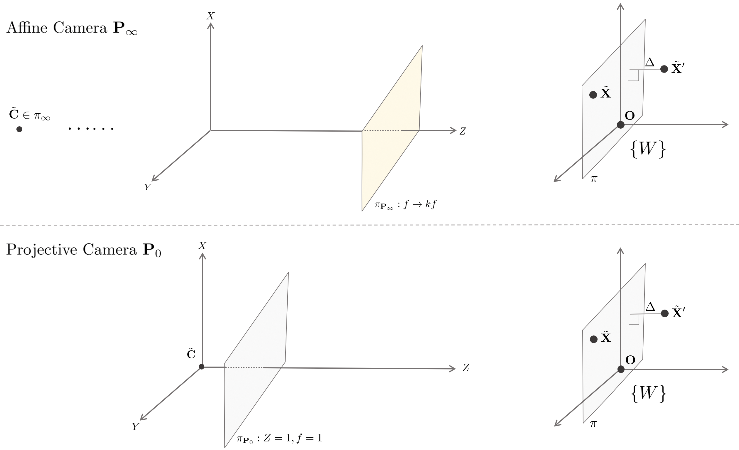
해당 섹션에서는 General Projective 카메라와 Affine 카메라로 동일한 물체를 찍었을 때 얼마나 큰 차이가 있는지에 대해서 설명한다. General Projective 카메라는 $\mathbf{P}_{0}$로 표기하고 Affine 카메라는 $\mathbf{P}_{\infty}$로 표기하며 시간 $t$에 따른 카메라 행렬의 변화는 $\mathbf{P}_{t}$로 표기한다.
월드 좌표계의 원점을 포함하면서 카메라 $\mathbf{P}_{t}$의 이미지 평면과 수직인 평면 $\pi$가 주어졌을 때 앞서 설명한 Vertigo Effect(zoom in + backward moving)을 수행하면 $\pi$에 위치한 점들은 $\mathbf{P}_{t}$에 의해 얻어지는 이미지 상의 점들이 $t$에 대하여 일정하다.
이를 증명해보면 평면 $\pi$ 상에 점 $\mathbf{X} \in \pi$가 주어졌을 때 $\pi$가 월드 좌표계의 원점을 포함하므로
\begin{equation}
\begin{aligned}
& \mathbf{X} = \begin{pmatrix} \alpha \mathbf{r}_{1,row} + \mathbf{\beta}\mathbf{r}_{2,row} \\ 1 \end{pmatrix} \in \mathbb{R}^{4}
\end{aligned}
\end{equation}
같이 나타낼 수 있다. 이를 $\mathbf{P}_{t}$를 통해 프로젝션하면
\begin{equation}
\begin{aligned}
\mathbf{P}_{t}\mathbf{X} & = \mathbf{K} \begin{bmatrix} \mathbf{r}_{1,row}^{\intercal} & -\mathbf{r}_{1,row}^{\intercal}\tilde{\mathbf{C}} \\ \mathbf{r}_{2,row}^{\intercal} & -\mathbf{r}_{2,row}^{\intercal}\tilde{\mathbf{C}} \\ d_{0}/d_{t} \cdot \mathbf{r}_{3,row} & d_{0} \end{bmatrix} \begin{bmatrix} \alpha \mathbf{r}_{1,row} + \beta \mathbf{r}_{2,row} \\ 1 \end{bmatrix} \\
& = \begin{bmatrix} * \\ * \\ d_{0} \end{bmatrix} \\
& \because \mathbf{r}_{1,row}\cdot \mathbf{r}_{3,row} = \mathbf{r}_{2,row}\cdot \mathbf{r}_{3,row}= 0 \
\end{aligned}
\end{equation}
따라서 월드 좌표계의 원점을 포함하는 평면 $\pi$ 상의 점 $\mathbf{X}$의 깊이(depth)는 $d_{0}$로 항상 일정하기 때문에 Vertigo Effect을 수행하면 시간 $t$에 관계없이 일정한 크기로 보인다. 즉, General Projective 카메라와 Affine 카메라에서 $\mathbf{X}$는 모두 동일한 이미지 상의 점으로 변환된다.
\begin{equation}
\begin{aligned}
\mathbf{P}_{0}\mathbf{X} = \mathbf{P}_{t}\mathbf{X} = \mathbf{P}_{\infty}\mathbf{X}
\end{aligned}
\end{equation}
만약 월드 좌표계 원점을 지나면서 이미지 평면과 수직인 평면 $\pi$ 상에 있는 점이 아닌, 평면 $\pi$로부터 거리가 $\Delta$ 만큼 떨어져 있는 월드 상의 점 $\mathbf{X}^{\prime}$를 두 카메라에서 찍는 경우 $\mathbf{P}_{0}\mathbf{X}^{\prime} \neq \mathbf{P}_{\infty}\mathbf{X}^{\prime}$가 된다. $\mathbf{X}^{\prime}$는 다음과 같이 나타낼 수 있다.
\begin{equation}
\begin{aligned}
\mathbf{X}^{\prime} = \begin{pmatrix} \alpha \mathbf{r}_{1,row} + \beta \mathbf{r}_{2,row} + \Delta \mathbf{r}_{3,row} \\ 1 \end{pmatrix}
\end{aligned}
\end{equation}
이 때, $\mathbf{r}_{3,row}$는 카메라의 주축(principal axis)를 의미한다. $\mathbf{X}^{\prime}$를 두 카메라에 프로젝션하면
\begin{equation}
\begin{aligned}
\mathbf{x}_{\text{proj}} & = \mathbf{P}_{0}\mathbf{X}^{\prime} = \mathbf{K}\begin{pmatrix} \tilde{x}\\\tilde{y}\\\tilde{z}_{\text{proj}} \end{pmatrix}
& = \mathbf{K}\begin{pmatrix}
\alpha - \mathbf{r}_{1,row}^{\intercal}\tilde{\mathbf{C}} \\
\beta - \mathbf{r}_{2,row}^{\intercal}\tilde{\mathbf{C}} \\
d_{0} + \Delta
\end{pmatrix}
\end{aligned}
\end{equation}
\begin{equation}
\begin{aligned}
\mathbf{x}_{\text{affine}} & = \mathbf{P}_{\infty}\mathbf{X}^{\prime} = \mathbf{K}\begin{pmatrix} \tilde{x}\\\tilde{y}\\\tilde{z}_{\text{affine}} \end{pmatrix}
& = \mathbf{K}\begin{pmatrix}
\alpha - \mathbf{r}_{1,row}^{\intercal}\tilde{\mathbf{C}} \\
\beta - \mathbf{r}_{2,row}^{\intercal}\tilde{\mathbf{C}} \\
d_{0}
\end{pmatrix}
\end{aligned}
\end{equation}
가 된다. $\tilde{z}_{\text{proj}}$는 다음과 같이 구할 수 있다.
\begin{equation}
\begin{aligned}
\tilde{z}_{\text{proj}} & = [\mathbf{r}_{3,row} | -\mathbf{r}_{3,row}\tilde{\mathbf{C}}]\mathbf{X}^{\prime} \\
& = [\mathbf{r}_{3,row} | -\mathbf{r}_{3,row}\tilde{\mathbf{C}}]\begin{pmatrix} \alpha \mathbf{r}_{1,row} + \beta \mathbf{r}_{2,row} + \Delta \mathbf{r}_{3,row} \\ 1 \end{pmatrix} \\
& = -\mathbf{r}_{3,row}\tilde{\mathbf{C}} + \Delta \\
& = d_{0} + \Delta
\end{aligned}
\end{equation}
카메라 캘리브레이션 행렬 $\mathbf{K}$는 다음과 같이 나타낼 수 있다.
\begin{equation}
\begin{aligned}
\mathbf{K} = \begin{bmatrix} \mathbf{K}_{2\times 2} & \tilde{\mathbf{x}}_{0} \\ \tilde{0}^{\intercal} & 1 \end{bmatrix}
\end{aligned}
\end{equation}
이 때, $\mathbf{K}_{2\times 2}$는 $2\times 2$ 크기의 상삼각(upper-triangular)행렬을 의미하고 $\tilde{\mathbf{x}}_{0} = \begin{pmatrix} x_{0} & y_{0} \end{pmatrix}^{\intercal}$는 이미지 평면의 원점을 의미한다. 이를 고려하여 위 공식들을 다시 정리해보면
\begin{equation}
\begin{aligned}
& \mathbf{x}_{\text{proj}} = \begin{pmatrix} \mathbf{K}_{2\times 2}\tilde{\mathbf{x}} + (d_{0}+\Delta)\tilde{\mathbf{x}}_{0} \\ d_{0} + \Delta \end{pmatrix} \\
& \mathbf{x}_{\text{affine}} = \begin{pmatrix} \mathbf{K}_{2\times 2}\tilde{\mathbf{x}} + d_{0}\tilde{\mathbf{x}}_{0} \\ d_{0} \end{pmatrix} \\
\end{aligned}
\end{equation}
와 같다. 이 때 $\tilde{\mathbf{x}} = \begin{pmatrix} \tilde{x} & \tilde{y} \end{pmatrix}^{\intercal}$를 의미한다. 두 점 $\mathbf{x}_{\text{proj}}$와 $\mathbf{x}_{\text{affine}}$의 Inhomogeneous 좌표를 계산해보면 마지막 항으로 나눈 값이 되므로
\begin{equation}
\begin{aligned}
& \tilde{\mathbf{x}}_{\text{proj}} = \tilde{\mathbf{x}}_{0} + \mathbf{K}_{2\times 2}\tilde{\mathbf{x}}/(d_{0}+\Delta) \\
& \tilde{\mathbf{x}}_{\text{affine}} = \tilde{\mathbf{x}}_{0} + \mathbf{K}_{2\times 2}\tilde{\mathbf{x}}/d_{0} \\
\end{aligned}
\end{equation}
가 된다. 결론적으로 General Projective 카메라와 Affine 카메라를 통해 프로젝션한 두 점의 차이는 다음과 같다.
\begin{equation}
\begin{aligned}
\tilde{\mathbf{x}}_{\text{affine}} - \tilde{\mathbf{x}}_{0} = \frac{d_{0}+\Delta}{d_{0}} (\tilde{\mathbf{x}}_{\text{proj}} - \tilde{\mathbf{x}}_{0})
\end{aligned}
\end{equation}
위 공식을 Discrepancy Equation이라고 부르며 $\Delta=0$인 경우, 월드 좌표계의 원점을 포함하면서 이미지 평면과 수직인 평면 $\pi$ 상의 점인 경우, 두 카메라를 통해 촬영한 물체는 동일한 이미지 상의 점으로 프로젝션된다는 것을 의미한다. 영화 Vertigo 또는 Jaws를 보면 이와 같은 현상을 볼 수 있는데 주인공의 얼굴이 변하지 않으면서 주변의 환경이 Zoom Out되는 것을 볼 수 있다.
3. Computation of the Camera Matrix $\mathbf{P}$
해당 섹션에서는 $\mathbb{P}^{3}$ 공간 상의 점 $\mathbf{X}_{i}$와 $\mathbb{P}^{2}$ 공간 상의 점 $\mathbf{x}_{i}$들의 대응쌍 $(\mathbf{x}_{i}, \mathbf{X}_{i})$ 여러개를 사용하여 카메라 행렬 $\mathbf{P}$를 수치적으로 구하는 방법에 대해 설명한다. 이러한 방법을 일반적으로 Resectioning 또는 Calibration이라고 부른다.
3.1. Basic equations
대응점 쌍 $(\mathbf{x}_{i}, \mathbf{X}_{i})$가 주어졌을 때 두 점 사이의 대응관계는 다음과 같다.
\begin{equation}
\begin{aligned}
\mathbf{x}_{i} = \mathbf{PX}_{i}
\end{aligned}
\end{equation}
이 때, $\mathbf{PX}_{i}$는
\begin{equation}
\begin{aligned}
\mathbf{PX}_{i} & = \begin{bmatrix} \mathbf{p}_{1,row}^{\intercal} \\ \mathbf{p}_{2,row}^{\intercal} \\ \mathbf{p}_{3,row}^{\intercal} \end{bmatrix}\mathbf{X}_{i}
& = \begin{bmatrix}
\mathbf{p}_{1,row}^{\intercal}\mathbf{X}_{i} \\
\mathbf{p}_{2,row}^{\intercal}\mathbf{X}_{i} \\
\mathbf{p}_{3,row}^{\intercal}\mathbf{X}_{i}
\end{bmatrix}
\end{aligned}
\end{equation}
와 같이 행벡터(row vector)를 사용하여 나타낼 수 있다. 이 때, $\mathbf{p}_{i,row} \in \mathbb{R}^{4\times 1}$인 벡터를 의미한다. $\mathbf{x} = \begin{pmatrix} x&y&w \end{pmatrix}^{\intercal}$라고 하면 $\mathbf{x}_{i} \times \mathbf{PX}_{i}=0$이므로
\begin{equation}
\begin{aligned}
\mathbf{x}_{i} \times \mathbf{PX}_{i} =
\begin{pmatrix}
y_{i}\cdot\mathbf{p}_{2,row}^{\intercal}\mathbf{X}_{i} - w_{i}\cdot\mathbf{p}_{3,row}\mathbf{X}_{i} \\
w_{i}\cdot\mathbf{p}_{1,row}^{\intercal}\mathbf{X}_{i} - x_{i}\cdot\mathbf{p}_{3,row}\mathbf{X}_{i} \\
x_{i}\cdot\mathbf{p}_{2,row}^{\intercal}\mathbf{X}_{i} - y_{i}\cdot\mathbf{p}_{1,row}\mathbf{X}_{i} \\
\end{pmatrix} = 0
\end{aligned}
\end{equation}
과 같다. 이를 $\mathbf{Ap} = 0$ 형태로 정리하면
\begin{equation}
\begin{aligned}
\begin{bmatrix}
\mathbf{0}^{\intercal} & -w_{i}\mathbf{X}_{i}^{\intercal} & y_{i}\mathbf{X}_{i}^{\intercal} \\
w_{i}\mathbf{X}_{i}^{\intercal} & \mathbf{0}^{\intercal} & -x_{i}\mathbf{X}_{i}^{\intercal} \\
-y_{i}\mathbf{X}_{i}^{\intercal} & x_{i}\mathbf{X}_{i}^{\intercal} & \mathbf{0}^{\intercal} \\
\end{bmatrix}
\begin{pmatrix} \mathbf{p}_{1,row} \\ \mathbf{p}_{2,row} \\ \mathbf{p}_{3,row} \end{pmatrix} = 0
\end{aligned}
\end{equation}
이 된다. 이 때 좌측 행렬의 마지막 행(row)은 선형의존이므로 첫 번째 행과 두 번째 행만 표현하면
\begin{equation}
\begin{aligned}
\underbrace{\begin{bmatrix}
\mathbf{0}^{\intercal} & -w_{i}\mathbf{X}_{i}^{\intercal} & y_{i}\mathbf{X}_{i}^{\intercal} \\
w_{i}\mathbf{X}_{i}^{\intercal} & \mathbf{0}^{\intercal} & -x_{i}\mathbf{X}_{i}^{\intercal} \\
\end{bmatrix}}_{\mathbf{A}}
\begin{pmatrix} \mathbf{p}_{1,row} \\ \mathbf{p}_{2,row} \\ \mathbf{p}_{3,row} \end{pmatrix} = 0
\end{aligned}
\end{equation}
과 같다. 이 때, 행렬 $\mathbf{A}$는 $\mathbb{R}^{2n\times 12}$크기이고 벡터 $\begin{pmatrix} \mathbf{p}_{1,row} \\ \mathbf{p}_{2,row} \\ \mathbf{p}_{3,row} \end{pmatrix}$는 $12\times1$ 크기이다. 위 방정식은 $\mathbf{Ap}=0$ 형태이므로 특이값 분해(SVD) 같은 방법을 통해 벡터 $\mathbf{p}$를 구할 수 있다.
3.1.1. Minimal solution
벡터 $\mathbf{p} \in \mathbb{R}^{12}$를 스케일을 제외하고(up to scale) 구하기 위해서는 총 11개의 식이 필요하다. 하나의 대응점 쌍 $(\mathbf{x}_{i}, \mathbf{X}_{i})$을 사용하면 2개의 식이 도출되므로 $\mathbf{p}$를 구하기 위해서는 최소 5.5개의 대응점 쌍이 필요하다. 노이즈가 없는 5.5개의 대응점 쌍이 주어진 경우 행렬 $\mathbf{A}$의 rank가 11가 되어 Null Space 벡터가 유일한 해 벡터 $\mathbf{p}$가 된다.
3.1.2. Over-determined solution
일반적으로 대응점 쌍 $(\mathbf{x}_{i}, \mathbf{X}_{i})$은 6개보다 훨씬 많은 개수를 얻을 수 있으며 데이터가 노이즈를 포함하고 있으므로 행렬 $\mathbf{A}$의 rank가 12가 된다. 따라서 Null Space가 존재하지 않으므로 해 벡터 $\mathbf{p}$를 구할 수 없다. 이러한 $\mathbf{Ap}=0$ 선형 시스템을 Over-determined 시스템이라고 하며 이 때는 $\|\mathbf{p} \|=1$인 경우에 대하여 $\|\mathbf{Ap} \|$의 크기가 최소가 되는 근사해 $\hat{\mathbf{p}}$를 구해야 한다.
3.1.3. Degenerate configurations
5.5개 이상의 대응점 쌍 $(\mathbf{x}_{i}, \mathbf{X}_{i})$이 서로 선형독립이 아닐 경우 유일한 해 벡터 $\mathbf{p}$를 결정할 수 없게 되고 이러한 대응점 쌍들을 Degenerate Configuration이라고 한다. 유일한 해 벡터 $\mathbf{p}$를 결정할 수 없다는 의미는 월드 상의 한 점 $\mathbf{X}$에 대하여
\begin{equation}
\begin{aligned}
& ^{\exists}\mathbf{P}^{\prime}, \ \ \mathbf{P} \neq \mathbf{P}^{\prime} \\
& \mathbf{PX}_{i} = \mathbf{P}^{\prime}\mathbf{X}_{i} \quad ^{\forall}i
\end{aligned}
\end{equation}
를 만족하는 임의의 다른 카메라 행렬 $\mathbf{P}^{\prime}$이 존재한다는 의미이다. 이는 특정 상수 $\theta$에 대해 $\mathbf{PX} = -\theta \mathbf{P}^{\prime}\mathbf{X}$ 또한 성립한다는 의미와 동일하므로 이를 정리하면
\begin{equation}
\begin{aligned}
\underbrace{(\mathbf{P} + \theta \mathbf{P}^{\prime})}_{\mathbf{P}_{\theta}}\mathbf{X} = 0 \quad \text{for some } \theta
\end{aligned}
\end{equation}
와 같고 $\mathbf{P}_{\theta}\mathbf{X}=0$을 만족하는 월드 상의 점 $\mathbf{X}$는 $\mathbf{P}$와 $\mathbf{P}^{\prime}$을 구분할 수 없다. 이와 같이 $\mathbf{P}, \mathbf{P}^{\prime}$에 의해 같은 이미지 평면 상의 점으로 옮겨지는 $\mathbf{X}$의 집합을 $\mathcal{S}_{\theta}$라고 하면
\begin{equation}
\begin{aligned}
\mathcal{S}_{\theta} = \{ \mathbf{X} \ | \ \mathbf{P}_{\theta}\mathbf{X}=0 \}
\end{aligned}
\end{equation}
$\mathcal{S}_{\theta}$를 만족하는 월드 상의 점 $\mathbf{X}$는 다음과 같다.
- 모든 $\mathbf{X}_{i}$들이 Twisted Cubic 상에 위치한 경우
- 모든 $\mathbf{X}_{i}$들이 동일한 평면 위에 존재하며 카메라 중심점을 포함한 직선 위에 존재하는 경우
Twisted Cubic이란 $\mathbb{P}^{3}$ 공간 상에 존재하는 곡선을 의미한다. Twisted Cubic $\mathbf{C}_{\theta}$으로 구성된 집합 $\mathcal{C}_{\theta}$는
\begin{equation}
\begin{aligned}
\mathcal{C}_{\theta} = \{ \mathbf{C}_{\theta} \ | \ \mathbf{P}_{\theta}\mathbf{C}_{\theta}=0 \ \text{ and } \mathbf{P}_{\theta} \text{'s rank is 3} \}
\end{aligned}
\end{equation}
을 만족하는 집합을 의미한다. 이 때, $\mathbf{C}_{\theta}$는 3차식의 형태로 나타나는데 중근으로 인해 Twisted Cubic이 아닌 경우도 있으나 일반적으로 Twisted Cubic을 의미한다. $\mathbf{P}_{\theta}\mathbf{C}_{\theta}=0$이고 $\mathbf{P}_{\theta}$의 rank가 3이므로 $\mathbf{C}_{\theta}$는 $\mathbf{P}_{\theta}$의 행공간(row space)에 들어가 있다는 의미가 된다.
\begin{equation}
\begin{aligned}
\mathbf{C}_{\theta} = \text{Row } \mathbf{P}_{\theta}
\end{aligned}
\end{equation}
따라서 $\mathbf{C}_{\theta} = \begin{pmatrix} c_{1}&c_{2}&c_{3}&c_{4} \end{pmatrix}$일 때
\begin{equation}
\begin{aligned}
\det \begin{pmatrix} c_{1}&c_{2}&c_{3}&c_{4} \\ -&-&-&- \\ -&\mathbf{P}_{\theta}&-&- \\ -&-&-&- \end{pmatrix} = 0
\end{aligned}
\end{equation}
이 성립한다. 이를 전개하면 $\det(2\ 3\ 4)c_{1} -\det(1\ 3\ 4)c_{2} + \det(1\ 2\ 4)c_{3} -\det(1\ 2\ 3)c_{4}=0$이 되고 이 때, $\det(a\ b\ c)$는 행렬 $\mathbf{P}_{\theta}$의 $a,b,c$ 행과 열의 서브행렬식(sub-determinant, subminor)를 의미한다. 이를 통해 $\mathbf{C}_{\theta}$를 다시 정리하면
\begin{equation}
\begin{aligned}
\mathbf{C}_{\theta} = (\det(2\ 3\ 4), -\det(1\ 3\ 4), \det(1\ 2\ 4), -\det(1\ 2\ 3))
\end{aligned}
\end{equation}
으로 나타낼 수 있고 각각의 항들이 전부 3차식인 Twisted Cubic이 된다. $\mathbf{P}, \mathbf{P}^{\prime}$에 따라 $\mathbf{C}_{\theta}$의 모든 항들이 공통근을 가질 수 있고 각 항들의 차수가 3차 이하로 떨어질 수 있다. 이러한 경우를 $\mathbf{C}_{\theta}$의 Degenerate Configuration이라고 부르며 이러한 $\mathbf{C}_{\theta}$는 Twisted Cubic이 아니다.
3.1.4. Line correspondences
월드 상의 한 직선 $\mathbf{L}$을 카메라 행렬 $\mathbf{P}$로 프로젝션하여 이미지 평면 상의 직선 $\mathbf{l}$을 얻었을 경우 점과 달리 직선은 $\mathbf{l} \neq \mathbf{PL}$이다.
\begin{equation}
\begin{aligned}
& \mathbf{x} = \mathbf{PX} \ \text{ but, } \ \mathbf{l} \neq \mathbf{PL} \\
\end{aligned}
\end{equation}
직선 $\mathbf{L}$ 상의 한 점 $\mathbf{X}$를 카메라에 프로젝션하여 얻은 점 $\mathbf{x}$는 직선 $\mathbf{l}$ 위에 존재하므로
\begin{equation}
\begin{aligned}
& \mathbf{l}^{\intercal}\mathbf{x} = \mathbf{l}^{\intercal}\mathbf{PX} = 0 \\
& \Rightarrow \mathbf{Ap} = 0
\end{aligned}
\end{equation}
와 같은 벡터 $\mathbf{p}$에 대한 선형 방정식이 성립한다. 따라서 월드 상의 직선 $\mathbf{L}$ 위에 존재하는 여러 점들 $\mathbf{X}_{i}$를 사용하면 벡터 $\mathbf{p}$에 대한 선형 방정식이 성립하여 이를 통해 카메라 행렬 $\mathbf{P}$를 구할 수 있다.
3.2. Geometric error
앞서 설명한 방법과 같이 대응점 쌍 $(\mathbf{x}_{i}, \mathbf{X}_{i})$를 이용하여 $\mathbf{Ap}=0$ 형태의 Over-determined 선형시스템을 구성한 후 $\| \mathbf{p} \|=1$이면서 $\| \mathbf{Ap} \|$의 크기를 최소화하는 근사해 벡터 $\hat{\mathbf{p}}$를 구할 수 있다. 해당 섹션에서는 더욱 정확한 카메라 행렬 $\mathbf{P}$를 구하기 위해 기하학적 에러(geometric error)를 최소화하는 방법에 대해 설명한다. 기하학적 에러는 이미지 평면 상에서 이미 주어진 $\mathbf{x}_{i}$와 월드 상의 점 $\mathbf{X}_{i}$를 프로젝션한 $\mathbf{PX}_{i}$ 사이의 픽셀 거리를 의미한다. 실제 데이터에서는 노이즈로 인해 $\mathbf{x}_{i} \neq \mathbf{PX}_{i}$이므로 두 점 사이의 거리 $d(\mathbf{x}_{i}, \mathbf{PX}_{i})$를 최소화해주는 최적의 카메라 행렬 $\mathbf{P}$를 찾아야 한다.
\begin{equation}
\begin{aligned}
\min_{\mathbf{P}} d(\mathbf{x}_{i}, \mathbf{PX}_{i})^{2}
\end{aligned}
\end{equation}
$d(\mathbf{x}_{i}, \mathbf{PX}_{i})^{2}$는 일반적으로 비선형이므로 비선형 최소제곱법(non-linear least squares) 방법들인 Gauss-Newton(GN) 또는 Levenberg-Marquardt(LM) 등과 같은 방법을 통해 최적의 카메라 행렬 $\mathbf{P}$를 구할 수 있다.
3.2.1. Algorithm 7.1
- Objective: 주어진 대응점 쌍 $(\mathbf{x}_{i}, \mathbf{X}_{i}),\ i=1,\cdots,6,\cdots$에 대하여 $\mathbf{P}$에 대한 MLE(maximum likelihook estimation) 값을 찾는다. 즉, $\sum_{i} d(\mathbf{x}_{i}, \mathbf{PX}_{i})^{2}$를 최소로하는 카메라 행렬 $\mathbf{P}$를 찾는다.
- Normalization: 이미지 포인트 $\mathbf{x}_{i}$를 정규화하는 행렬 $\mathbf{T}$를 통해 $\mathbf{x}_{i} \rightarrow \bar{\mathbf{x}}_{i}$로 정규화시키고 월드 상의 점 $\mathbf{X}_{i}$를 정규화하는 행렬 $\mathbf{U}$를 통해 $\mathbf{X}_{i} \rightarrow \bar{\mathbf{X}}_{i}$로 정규화시킨다. 정규화를 수행하지 않고 DLT(direct linear transformation)을 수행하는 경우 $\mathbb{P}^{2}, \mathbb{P}^{3}$ 공간의 특성 상 마지막 항의 값이 1로 매우 작고 나머지 항들은 매우 크므로 정상적인 해가 도출되지 않는다.
- DLT: 정규화된 대응점 쌍들을 앞서 설명한 Over-determined 시스템 $\bar{\mathbf{A}}\bar{\mathbf{p}}=0$으로 구성한다. 다음으로 $\|\bar{\mathbf{p}} \|=1$이며 $\|\bar{\mathbf{A}}\bar{\mathbf{p}}\|$를 최소화하는 근사해 $\bar{\mathbf{p}}$를 DLT를 통해 구한 후 이를 초기값 $\bar{\mathbf{P}}_{0}$으로 설정한다.
- Minimize geometric error: 다음과 같은 기하학적 에러를 GN 또는 LM 방법을 통해 최소화하여 최적의 정규화된 카메라 행렬 $\bar{\mathbf{P}}$를 계산한다.
\begin{equation}
\begin{aligned}
\min_{\bar{\mathbf{P}}}\sum_{i} d(\bar{\mathbf{x}}_{i}, \bar{\mathbf{P}}\bar{\mathbf{X}}_{i})^{2} \quad \text{ start at } \bar{\mathbf{P}}_{0}
\end{aligned}
\end{equation}
- Denormalization: 정규화된 카메라 행렬을 다시 원래 카메라 행렬로 복원한다.
\begin{equation}
\begin{aligned}
\mathbf{P} = \mathbf{T}^{-1}\bar{\mathbf{P}}\mathbf{U}
\end{aligned}
\end{equation}
위 알고리즘을 일반적으로 The Gold Standard algorithm for estimating $\mathbf{P}$라고 한다. 실제로 위 알고리즘을 사용할 때는 임의의 대응점 쌍을 사용하는 것이 아니고 체크보드 상의 대응점 쌍을 사용한다. 이렇게 체크보드를 통해 카메라 행렬 $\mathbf{P}$를 추정하는 알고리즘을 Zhang's Method라고 한다.
3.3. Zhang's method
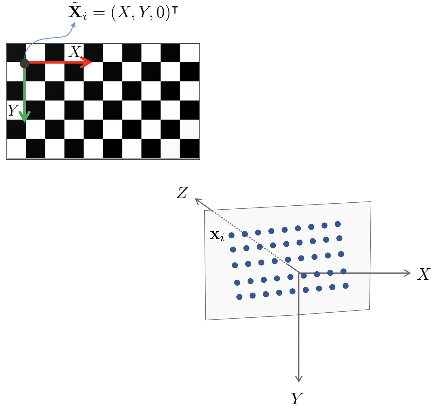
실제로 Gold Standard 알고리즘을 사용할 때는 임의의 대응점 쌍을 사용하는 것이 아닌 체커보드 상의 대응점 쌍을 사용한다. 이렇게 체커보드를 통해 카메라 행렬 $\mathbf{P}$를 추정하는 알고리즘을 Zhang's Method[2]라고 한다. 월드 상의 체커보드 평면 $\pi_{0}$가 주어졌을 때 월드 상의 원점을 체커보드의 좌측 상단으로 설정하고 체커보드의 평면이 $Z=0$인 평면으로 설정한다.
\begin{equation}
\begin{aligned}
\pi_{0} = \{ \mathbf{X}=(X,Y,Z)^{\intercal} \ | \ Z=0 \}
\end{aligned}
\end{equation}
이에 따라 체커보드 평면 $\pi_{0}$위의 임의의 점 $\mathbf{X}_{i}$들은 $Z=0$인 점이 된다.
\begin{equation}
\begin{aligned}
\mathbf{X}_{i} = (\ast,\ \ast,\ 0)^{\intercal}
\end{aligned}
\end{equation}
체커보드 상의 한 점 $\mathbf{X}=(X,\ Y,\ 0,\ 1)^{\intercal}$를 프로젝션하면
\begin{equation}
\begin{aligned}
\mathbf{PX} & = \mathbf{P} \begin{pmatrix} X\\Y\\0\\1 \end{pmatrix} = \mathbf{K}[\mathbf{R} \ | \ \mathbf{t}] \begin{pmatrix} X\\Y\\0\\1 \end{pmatrix} \\
& = \mathbf{K}[\mathbf{r}_{1,col} \ \mathbf{r}_{2,col} \ \mathbf{t}]\mathbf{X}
\end{aligned}
\end{equation}
가 된다. $z=0$이므로 행렬 $\mathbf{R}$의 세 번째 열벡터(column vector)는 0이 된다. 행렬 $\mathbf{K}[\mathbf{r}_{1,col} \ \mathbf{r}_{2,col} \ \mathbf{t}] \in \mathbb{R}^{3\times 3}$는 체커보드 평면 $\pi_{0}$에서 이미지 평면 $\pi$로 변환하는 Homography $\mathbf{H}$로 볼 수 있다.
\begin{equation}
\begin{aligned}
\mathbf{H} = \mathbf{K}[\mathbf{r}_{1,col} \ \mathbf{r}_{2,col} \ \mathbf{t}]
\end{aligned}
\end{equation}
체커보드는 패턴의 길이와 갯수를 모두 알고 있기 때문에 자동적으로 체커보드 평면 $\pi_{0}$ 상의 점 $\mathbf{x}_{i},i=1,\cdots$를 알 수 있다. 다음으로 Feature Extraction 알고리즘을 사용하면 이미지 평면 $\pi$ 상에서 본 $\pi_{0}$의 점 $\mathbf{x}^{\prime}_{i}, i=1,\cdots$들을 알 수 있다. 따라서 대응점 쌍 $\mathbf{x}_{i} \in \pi_{0} \leftrightarrow \mathbf{x}_{i}^{\prime} \in \pi$을 얻을 수 있다. 이를 통해 $\pi_{0} \mapsto \pi$로 가는 Homography $\mathbf{H}$를 계산해보면
\begin{equation}
\begin{aligned}
& \mathbf{H} = \begin{bmatrix} \mathbf{h}_{1,col} & \mathbf{h}_{2,col} & \mathbf{h}_{3,col} \end{bmatrix} = \mathbf{K} \begin{bmatrix} \mathbf{r}_{1,col} & \mathbf{r}_{2,col} & \mathbf{t} \end{bmatrix} \\
\end{aligned}
\end{equation}
가 된다. 이를 정리하면
\begin{equation}
\begin{aligned}
& \mathbf{K}^{-1}\begin{bmatrix} \mathbf{h}_{1,col} & \mathbf{h}_{2,col} & \mathbf{h}_{3,col} \end{bmatrix} = \begin{bmatrix} \mathbf{r}_{1,col} & \mathbf{r}_{2,col} & \mathbf{t} \end{bmatrix}
\end{aligned}
\end{equation}
가 된다. 이 때, 직교행렬 $\mathbf{R}$의 열벡터인 $\mathbf{r}_{1,col}$과 $\mathbf{r}_{2,col}$은 서로 직교하므로 $\mathbf{r}_{1,col}^{\intercal}\mathbf{r}_{2,col}=0$이 성립한다. 해당 제약조건을 이용하면 $\mathbf{K}^{-1}\mathbf{h}_{1,col} = \mathbf{r}_{1,col}$이고 $\mathbf{K}^{-1}\mathbf{h}_{2,col} = \mathbf{r}_{2,col}$이므로 직교조건에 의해
\begin{equation}
\label{eq:1386}
\begin{aligned}
\mathbf{h}_{1,col}^{\intercal}\mathbf{K}^{-\intercal}\mathbf{K}^{-1}\mathbf{h}_{2,col} = 0
\end{aligned}
\end{equation}
이 성립한다. 또한 직교행렬 조건에 의해 스케일을 제외하고(up to scale) $\mathbf{r}_{1,col}^{\intercal}\mathbf{r}_{1,col} = \mathbf{r}_{2,col}^{\intercal}\mathbf{r}_{2,col}$이므로
\begin{equation}
\label{eq:1395}
\begin{aligned}
& \mathbf{h}_{1,col}^{\intercal}\mathbf{K}^{-\intercal}\mathbf{K}^{-1}\mathbf{h}_{1,col} = \mathbf{h}_{2,col}^{\intercal}\mathbf{K}^{-\intercal}\mathbf{K}^{-1}\mathbf{h}_{2,col}
\end{aligned}
\end{equation}
공식이 성립한다. 한 개의 체커보드 사진으로 부터 위와 같은 두 개의 방정식을 얻을 수 있다. 일반적인 카메라 캘리브레이션 행렬 $\mathbf{K}$는
\begin{equation}
\begin{aligned}
\mathbf{K} = \begin{bmatrix} f_{x} & s & x_{0} \\ & f_{y} & y_{0} \\ &&1 \end{bmatrix}
\end{aligned}
\end{equation}
과 같이 5개의 변수를 가지고 있으므로 $\mathbf{K}^{-\intercal}\mathbf{K}^{-1}$ 또한 5개의 변수를 가지고 있는 행렬이 된다. 따라서 최소 세 개 이상의 Homography $\mathbf{H}_{j}, \ j=1,2,3$가 주어졌을 때 $\mathbf{K}^{-\intercal}\mathbf{K}^{-1}$를 결정할 수 있다.
- 5개의 파라미터를 갖고 있는 행렬 $\mathbf{K}$를 구하기 위해 최소 세 개 이상의 체커보드 이미지를 획득한다. 하나의 이미지 당 두 개의 방정식을 얻을 수 있으므로 세 장 이상을 획득해야 한다. 각각의 이미지마다 Homography $\mathbf{H}_{j},\ j=1,2,3$을 구할 수 있고 공식 \eqref{eq:1386}, \eqref{eq:1395}를 구한다.
- $\mathbf{S} =\mathbf{K}^{-\intercal}\mathbf{K}^{-1}$로 설정한다. 행렬 $\mathbf{S}$에 Cholesky Decomposition 또는 특이값 분해(SVD)를 수행하여 $\mathbf{K}^{-1}$을 구한다. 행렬 $\mathbf{S}$는 대칭이면서 Positivie Definite 행렬이므로 $\mathbf{U}^{\intercal}\mathbf{DU}$와 같이 분해되며 대각행렬 $\mathbf{D}$의 제곱근 행렬이 존재한다.
\begin{equation}
\begin{aligned}
\text{SVD}(\mathbf{S}) = \mathbf{U}^{\intercal}\mathbf{D}\mathbf{U} = (\mathbf{U}\sqrt{\mathbf{D}})(\mathbf{U}\sqrt{\mathbf{D}})^{\intercal}
\end{aligned}
\end{equation}
이를 통해 $\mathbf{K}$를 구할 수 있다.
- $\mathbf{K}^{-1}\mathbf{H} = [\mathbf{r}_{1,col} \ \mathbf{r}_{2,col} \ \mathbf{t}]$ 식을 통해 $\mathbf{r}_{1,col}, \mathbf{r}_{2,col}, \mathbf{t}$를 구한 다음
\begin{equation}
\begin{aligned}
\mathbf{r}_{3,col} = \mathbf{r}_{1} \times \mathbf{r}_{2}
\end{aligned}
\end{equation}
를 통해 구한다. 결론적으로 각각의 Homography $\mathbf{H}_{j},\ j=1,2,3$을 통해 카메라의 회전 $\mathbf{R}$과 이동 $\mathbf{t}$ 그리고 내부 파라미터 행렬 $\mathbf{K}$를 구할 수 있다.
3.4. Radial distortion
실제 카메라 이미지는 이상적인 핀홀 카메라 모델과 다르게 방사형 왜곡(radial distortion)을 포함하고 있기 때문에 이를 바로 캘리브레이션하면 정확한 $\mathbf{R},\mathbf{t},\mathbf{K}$를 구할 수 없다. 실제 툴킷을 사용하여 캘리브레이션을 수행해보면 앞서 구한 $\mathbf{R},\mathbf{t},\mathbf{K}$ 외에도 Distortion 파라미터들을 구할 수 있다. 해당 파라미터들이 이미지의 방사형 왜곡을 보정해주는 파라미터들이다.
초점거리(focal length) $f$가 작은 경우 Field of View(FOV)가 넓어지고 이 때 이미지의 가장자리 부근에서 방사형 왜곡이 크게 발생한다. 반대로 초점거리 $f$가 작으면 FOV가 작아지고 왜곡이 상대적으로 덜 발생한다.
왜곡이 존재하는 이미지 평면 상에서 한 점을 $(\breve{u}, \breve{v})$라고 하고 왜곡이 보정된 이미지 평면 상의 점을 $(u,v)$라고 하자. 두 점들의 단위는 $[pixel]$이다. 그리고 정규화된 이미지 평면(normalized image plane) 상의 왜곡이 존재하는 한 점을 $(\breve{x}, \breve{y})$라고 하고 왜곡이 보정된 점을 $(x,y)$라고 하자. 두 정규화된 점들의 단위는 $[mm]$이다. 정규화되었다는 말의 의미는 이미지 평면의 원점 $u_{0}, v_{0}$가 모두 0이라는 의미이다. 정규화된 점들 사이에는
\begin{equation}
\begin{aligned}
& \breve{x} = x + x(k_{1}r^{2} + k_{2}r^{4}) \\
& \breve{y} = y + y(k_{1}r^{2} + k_{2}r^{4}) \quad \text{where, } r^{2} = x^{2} + y^{2}
\end{aligned}
\end{equation}
가 성립한다. $r^{2}$ 값은 원점에서 거리가 멀어질 수록 왜곡이 크게 발생하는 것을 의미한다. 해당 정규화된 점들을 픽셀 단위 이미지 평면 상의 점들로 다시 표현하면
\begin{equation}
\begin{aligned}
& \breve{u} = u_{0} + \alpha \breve{x} \\
& \breve{v} = v_{0} + \beta \breve{v} \\
\end{aligned}
\end{equation}
가 된다. 이 때 $u_{0}, v_{0}$는 이미지 평면의 원점을 의미하며 $\alpha, \beta$는 mm 단위의 점들을 pixel 단위로 변환해주는 계수를 의미한다. 따라서 방사형 왜곡 파라미터 $k_{1}, k_{2}$를 구함으로써 왜곡된 점들과 실제 점들 사이의 관계를 알 수 있다.
4. More Single View Geometry
4.1. Camera calibration and the image of the absolute conic
4.1.1. Result 8.15
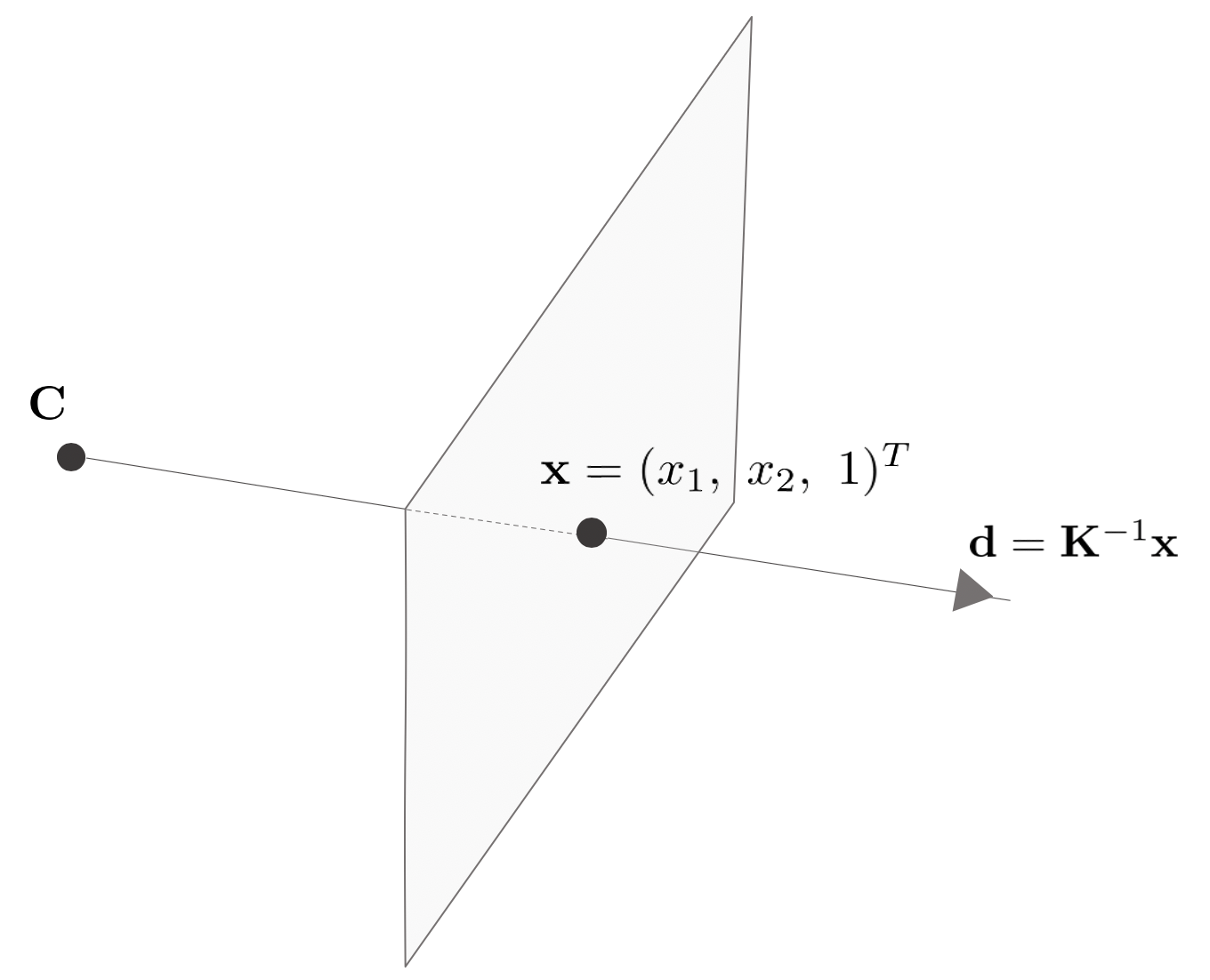
원점에 위치한 카메라 $\mathbf{C}$가 있을 때 한 점 $\mathbf{x}$를 Back-projection하면 카메라 중심을 지나는 직선 $\mathbf{d}$가 생성되는데 이 때, $\mathbf{d} = \mathbf{K}^{-1}\mathbf{x}$의 관계를 가진다.
\begin{equation}
\begin{aligned}
\mathbf{x} & = \mathbf{P} \begin{bmatrix} \lambda \mathbf{d} \\ 1 \end{bmatrix} \\
& = \mathbf{K} [ \mathbf{I} | 0 ] \begin{bmatrix} \lambda \mathbf{d} \\ 1 \end{bmatrix} = \mathbf{Kd} \\
\end{aligned}
\end{equation}
따라서 다음의 공식이 성립한다.
\begin{equation}
\begin{aligned}
& \mathbf{x} = \mathbf{Kd} \\
& \mathbf{d} = \mathbf{K}^{-1}\mathbf{x}
\end{aligned}
\end{equation}
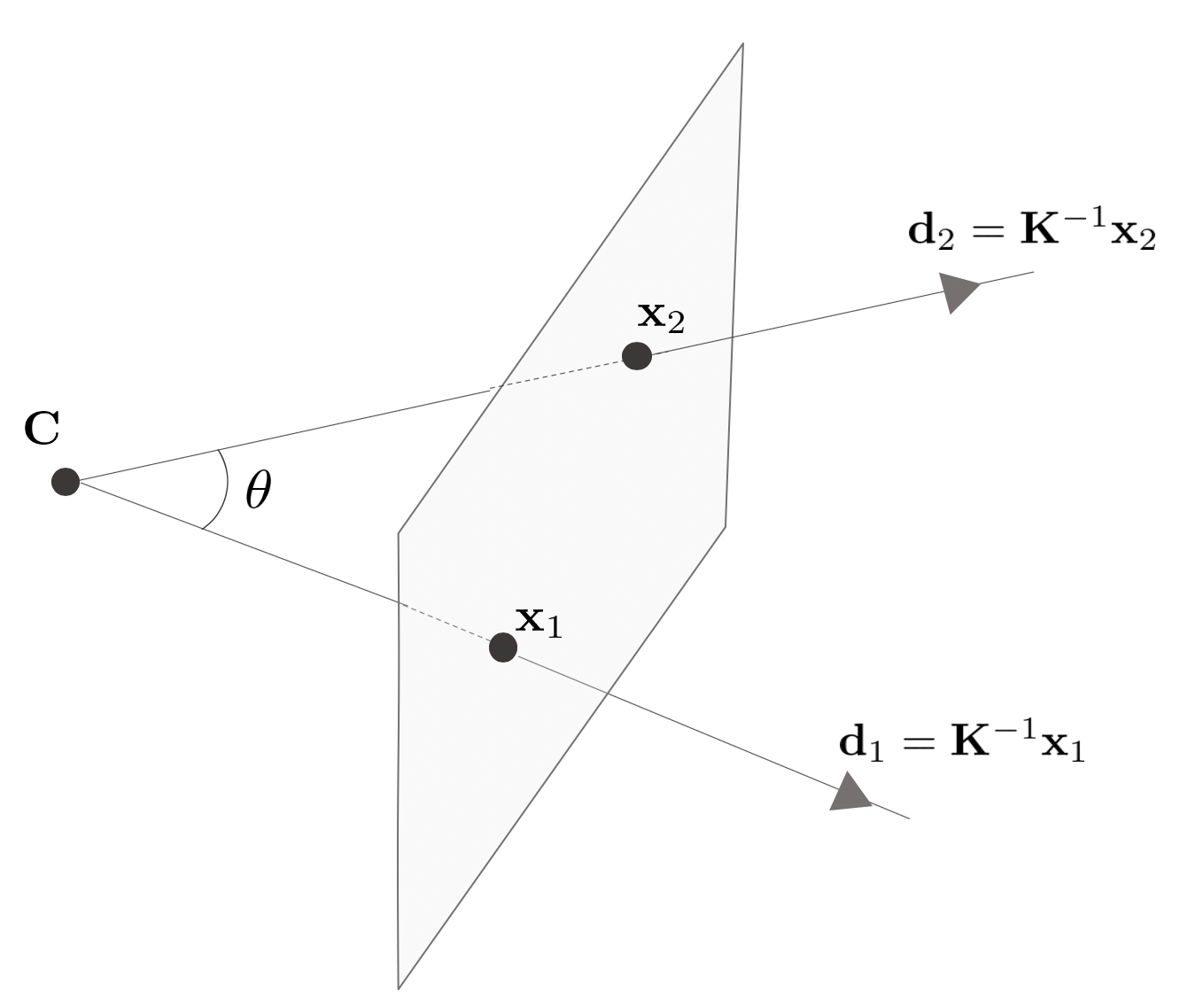
이미지 평면 상의 두 점 $\mathbf{x}_{1}, \mathbf{x}_{2}$를 Back-projection하면 각각 $\mathbf{d}_{1}, \mathbf{d}_{2}$의 직선이 생성되는데 이 때 두 직선이 이루는 각도는 다음과 같이 계산할 수 있다.
\begin{equation}
\begin{aligned}
\cos\theta & = \frac{\mathbf{d}_{1}^{\intercal}\mathbf{d}_{2}}{\sqrt{\mathbf{d}_{1}^{\intercal}\mathbf{d}_{1}}\sqrt{\mathbf{d}_{2}^{\intercal}\mathbf{d}_{2}}} = \frac{(\mathbf{K}^{-1}\mathbf{x}_{1})^{\intercal}(\mathbf{K}^{-1}\mathbf{x}_{2})}{\sqrt{(\mathbf{K}^{-1}\mathbf{x}_{1})^{\intercal}(\mathbf{K}^{-1}\mathbf{x}_{1})}\sqrt{(\mathbf{K}^{-1}\mathbf{x}_{2})^{\intercal}(\mathbf{K}^{-1}\mathbf{x}_{2})}} \\
& = \frac{\mathbf{x}_{1}^{\intercal}(\mathbf{K}^{-\intercal}\mathbf{K}^{-1})\mathbf{x}_{2}}{\sqrt{\mathbf{x}_{1}^{\intercal}\mathbf{K}^{-\intercal}\mathbf{K}^{-1}\mathbf{x}_{1}}\sqrt{\mathbf{x}_{2}^{\intercal}\mathbf{K}^{-\intercal}\mathbf{K}^{-1}\mathbf{x}_{2}}}
\end{aligned}
\end{equation}
이 때, $\mathbf{K}^{-\intercal}\mathbf{K}^{-1}$은 Image of Absolute Conic 을 의미한다.
4.1.2. Result 8.16
이미지 평면에 있는 직선 $\mathbf{l}$ 위에 한 점 $\mathbf{x}$가 위치할 때, 점과 직선 사이에는 다음 공식이 성립한다.
\begin{equation}
\begin{aligned}
\mathbf{x}^{\intercal}\mathbf{l} =0
\end{aligned}
\end{equation}
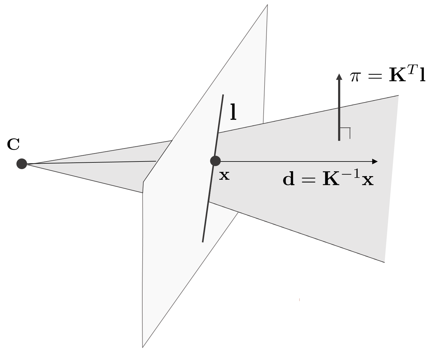
이 때, $\mathbf{l}$를 Back-projection하면 평면 $\pi$가 생성되고 $\mathbf{x}$를 Back-projection하면 $\mathbf{d}=\mathbf{K}^{-1}\mathbf{x}$가 생성되는데 평면 $\pi$와 직선 $\mathbf{d}$ 사이에는 $(\mathbf{K}^{-1}\mathbf{x})^{\intercal}\pi = 0$이 성립하고 이를 정리하면 $\mathbf{x}^{\intercal}(\mathbf{K}^{-\intercal}\pi)=0$가 성립한다. $\mathbf{x}^{\intercal}\mathbf{l}=0$의 공식에 따라 결론적으로 다음 공식이 성립한다.
\begin{equation}
\begin{aligned}
& \mathbf{K}^{-\intercal}\pi = \mathbf{l} \\
& \pi = \mathbf{K}^{\intercal}\mathbf{l}
\end{aligned}
\end{equation}
4.2. The image of the absolute conic
무한대 평면 $\pi_{\infty}$가 있을 때 $\pi_{\infty}$ 위에 위치한 무한대 점 $\mathbf{X}_{\infty} = (\mathbf{d}^{\intercal}, 0)^{\intercal}$이 있다고 하면 이를 카메라 $\mathbf{P}=\mathbf{KR}[\mathbf{I}|-\tilde{\mathbf{C}}]$에 프로젝션시키면 다음과 같다.
\begin{equation}
\begin{aligned}
\mathbf{x} = \mathbf{PX}_{\infty} = \mathbf{KR}[\mathbf{I} | -\tilde{\mathbf{C}}] \begin{bmatrix} \mathbf{d} \\0 \end{bmatrix} = \mathbf{KRd}
\end{aligned}
\end{equation}
즉, 무한대 평면 $\pi_{\infty}$ 위의 점 $\mathbf{d}$에 대해 $\mathbf{x} = \mathbf{Hd}$인 Homography가 존재한다고 했을 때 Homography $\mathbf{H}$는 $\mathbf{H}=\mathbf{KR}$과 같다. 무한대에 위치한 Absolute Conic $\Omega_{\infty}$는 $\mathbf{I}_{3}\in \pi_{\infty}$이다. $\Omega_{\infty}$를 Homography 변환하면
\begin{equation}
\begin{aligned}
\mathbf{H}(\Omega_{\infty}) & = \mathbf{H}^{-\intercal}\mathbf{I}_{3}\mathbf{H}^{-1} \\
& = (\mathbf{KR})^{-\intercal}\mathbf{I}_{3}(\mathbf{KR})^{-1} \\
& = \mathbf{K}^{-\intercal}\mathbf{R}^{-\intercal}\mathbf{R}^{-1}\mathbf{K}^{-1} \\
& = \mathbf{K}^{-\intercal}\mathbf{K}^{-1}
\end{aligned}
\end{equation}
4.2.1. Result 8.17
이에 따라 Image of Absolute Conic $\mathbf{w} = \mathbf{K}^{-\intercal}\mathbf{K}^{-1}$ 이 된다.
이미지 상의 두 점 $\mathbf{x}_{1}, \mathbf{x}_{2}$를 Back-projection 했을 때, 두 직선이 이루는 각도는
\begin{equation}
\begin{aligned}
\cos\theta = \frac{\mathbf{x}_{1}^{\intercal}\mathbf{w}\mathbf{x}_{2}}{\sqrt{\mathbf{x}_{1}^{\intercal}\mathbf{w}\mathbf{x}_{1}}\sqrt{\mathbf{x}_{2}^{\intercal}\mathbf{w}\mathbf{x}_{2}}}
\end{aligned}
\end{equation}
가 되고 이를 Homography 변환하면
\begin{equation}
\begin{aligned}
\cos\theta = \frac{(\mathbf{Hx}_{1})^{\intercal}\mathbf{H}^{-\intercal}\mathbf{w}\mathbf{H}^{-1}(\mathbf{Hx}_{2})}{\sqrt{\ast}\sqrt{\ast}}
\end{aligned}
\end{equation}
이 되므로 Homography 변환을 해도 두 각도는 여전히 보존된다. 만약 두 직선 $\mathbf{K}^{-1}\mathbf{x}_{1}$과 $\mathbf{K}^{-1}\mathbf{x}_{2}$가 직교하는 경우 다음 공식이 성립한다.
\begin{equation}
\begin{aligned}
\mathbf{x}_{1}^{\intercal}\mathbf{w}\mathbf{x}_{2} = 0
\end{aligned}
\end{equation}
4.3. Orthogonality and $\mathbf{w}$
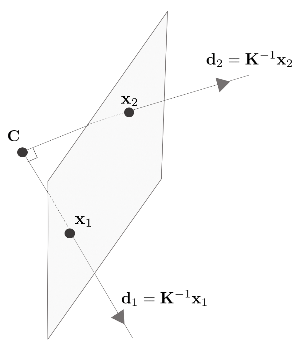
이미지 평면 상의 두 점 $\mathbf{x}_{1}, \mathbf{x}_{2}$를 Back-projection하면 두 직선 $\mathbf{K}^{-1}\mathbf{x}_{1}, \mathbf{K}^{-1}\mathbf{x}_2$가 생성된다. 만약 두 직선이 직교하는 경우 $\mathbf{x}_{1}^{\intercal}\mathbf{w}\mathbf{x}_{2}=0$의 공식이 성립한다. 그리고 $\mathbf{x}_{1}$가 직선 $\mathbf{l}$에 포함되어 있으면 $\mathbf{x}_{1}^{\intercal}\mathbf{l}=0$이 성립한다.
4.3.1. Result 8.19
위 두 공식을 결합하면
\begin{equation}
\begin{aligned}
& \mathbf{x}_{1}^{\intercal}\mathbf{w}\mathbf{x}_{2}=0 \\
& \mathbf{x}_{1}^{\intercal}\mathbf{l} = 0 \\
& \therefore \mathbf{l} = \mathbf{wx}_{2}
\end{aligned}
\end{equation}
4.4. Vanishing points and vanishing lines
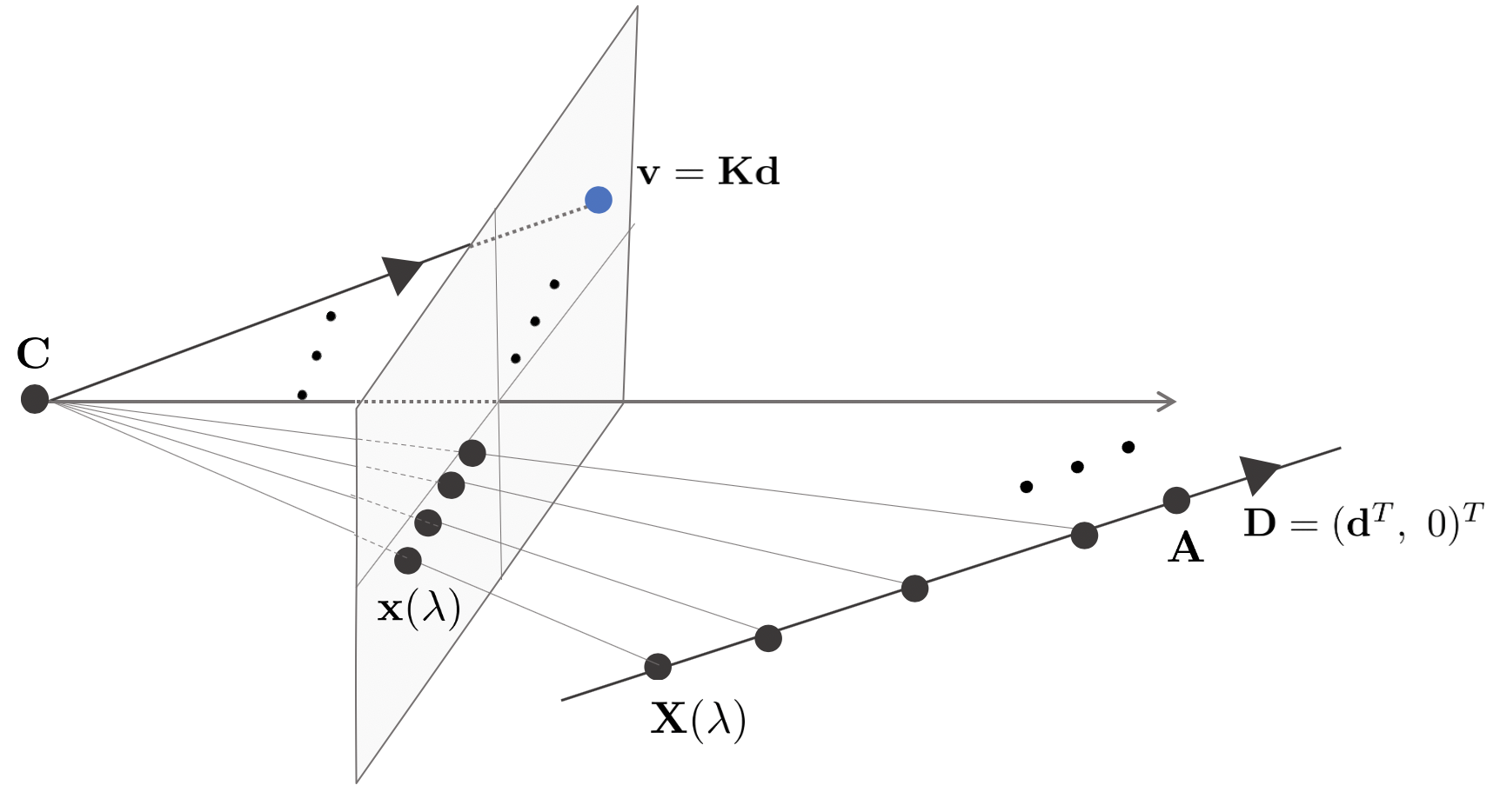
3차원 공간 상의 점 $\mathbf{A}$와 직선의 방향 $\mathbf{D}=(\mathbf{d}^{\intercal},0)^{\intercal}$가 존재할 때 직선 위에 존재하는 점 $\mathbf{X}(\lambda)$는 다음과 같이 정의된다.
\begin{equation}
\begin{aligned}
\mathbf{X}(\lambda) = \mathbf{A} + \lambda \mathbf{D} = \begin{bmatrix} \tilde{\mathbf{A}} + \lambda \mathbf{d} \\ 1 \end{bmatrix}
\end{aligned}
\end{equation}
점 $\mathbf{X}(\lambda)$를 이미지 평면에 프로젝션한 점 $\mathbf{x}(\lambda) = \mathbf{PX}(\lambda), \ \ \text{where } \ \mathbf{P} = \mathbf{K}[\mathbf{I}|0]$는 다음과 같이 정의된다.
\begin{equation}
\begin{aligned}
\mathbf{x}(\lambda) = \mathbf{PX}(\lambda) = \mathbf{PA} + \lambda \mathbf{PD} = \mathbf{a} + \lambda \mathbf{Kd}
\end{aligned}
\end{equation}
이 때, $\mathbf{a}$는 Image of $\mathbf{A}$를 의미한다.
4.4.1. Result 8.20
결론적으로 소실점(vanishing point) $\mathbf{v}$는 다음과 같이 정의된다.
\begin{equation}
\begin{aligned}
& \mathbf{v} = \lim_{\lambda \rightarrow \infty}\mathbf{x}(\lambda) = \lim_{\lambda \rightarrow \infty}(\mathbf{a} + \lambda \mathbf{Kd}) = \mathbf{Kd} \\
& \mathbf{v} = \mathbf{Kd}
\end{aligned}
\end{equation}
4.4.2. Camera rotation from vanishing points
소실점을 사용하여 카메라의 회전을 계산할 수 있다. 이미지 1에서 추출한 소실점 $\mathbf{v}_{1}$과 이미지 2에서 추출한 소실점 $\mathbf{v}_{2}$이 있을 때, $\mathbf{v}_{1}$의 방향은 $\mathbf{d}_{1} = \mathbf{K}^{-1}\mathbf{v}_{1}$이 되고 $\mathbf{v}_{2}$의 방향은 $\mathbf{d}_{2} = \mathbf{K}^{-1}\mathbf{v}_{2}$가 된다.
$\mathbf{K}, \mathbf{v}_{1}, \mathbf{v}_{2}$의 값을 모두 알고 있다고 가정하면 $\mathbf{d}_{1}, \mathbf{d}_{2}$의 값을 계산할 수 있게 되고 두 방향벡터는 다음과 같은 관계를 가진다.
\begin{equation}
\begin{aligned}
\mathbf{d}_{2} = \mathbf{Rd}_{1}
\end{aligned}
\end{equation}
이 때, 회전행렬 $\mathbf{R}$의 자유도는 3이므로 2개 이상의 소실점 쌍을 사용하면 회전행렬을 복원할 수 있다.
4.5. Vanishing Lines
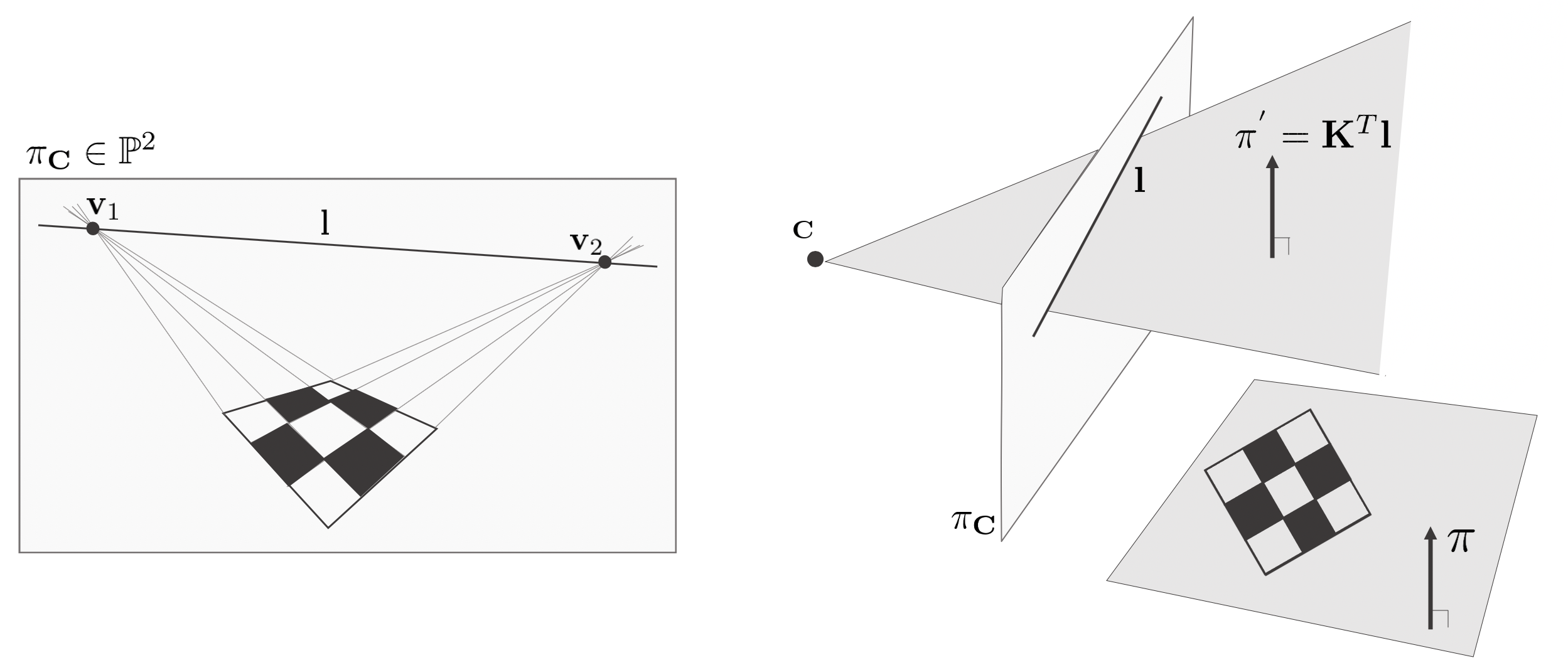
두 개 이상의 소실점(vanishing point) $\mathbf{v}_{i}, i=1,2,\cdots$ 들을 이어준 직선을 소실선(vanishing line) $\mathbf{l}$이라고 한다. 예를 들어 이미지 상의 체크보드가 있고 이로 인해 2개의 소실점 $\mathbf{v}_{1}, \mathbf{v}_{2}$를 구한 경우를 생각해보자. 이 경우, 두 소실점 $\mathbf{v}_{1},\mathbf{v}_{2}$를 이어주는 직선 $\mathbf{l}$을 체크보드 평면 $\pi$의 소실선이라고 한다.
\begin{equation}
\begin{aligned}
\mathbf{l} = \text{image of } \pi \cap \pi_{\infty}
\end{aligned}
\end{equation}
결론적으로 소실선 $\mathbf{l}$은 카메라 중심을 포함하고 체크보드 평면 $\pi$과 평행인 평면 $\pi^{\prime}$와 이미지 평면의 교집합을 의미한다. $\pi^{\prime}$은 소실선 $\mathbf{l}$을 Back-projection함으로써 계산할 수 있다. 이 때 평면과 직선의 관계에 따라
\begin{equation}
\begin{aligned}
\pi^{\prime} = \mathbf{K}^{\intercal}\mathbf{l}
\end{aligned}
\end{equation}
과 같이 계산할 수 있다.
4.6. Orthogonality relationships amongst vanishing points and lines
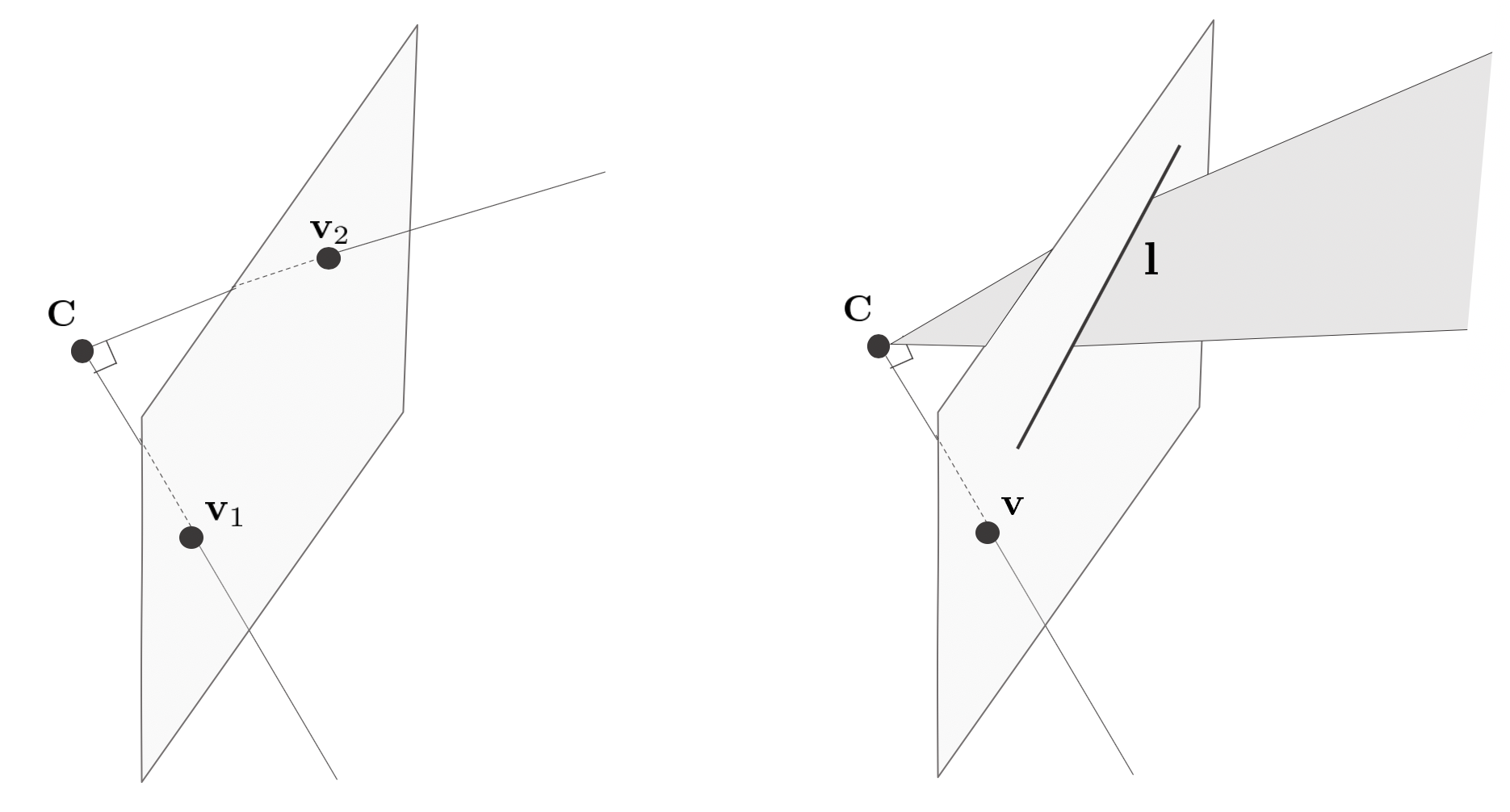
이미지 평면에서 두 개의 소실점 $\mathbf{v}_{1}, \mathbf{v}_{2}$을 Back-projection한 직선들이 서로 직교하는 조건은 다음과 같다.
\begin{equation}
\begin{aligned}
\mathbf{v}_{1}^{\intercal}\mathbf{w}\mathbf{v}_{2} = 0
\end{aligned}
\end{equation}
이 때, $\mathbf{w} = \mathbf{K}^{-\intercal}\mathbf{K}^{-1}$은 Image of Absolute Conic이다.
이미지 평면에서 소실점 $\mathbf{v}$을 Back-projection한 직선과 소실선 $\mathbf{l}$을 Back-projection한 평면이 직교하는 조건은 다음과 같다.
\begin{equation}
\begin{aligned}
\mathbf{l} = \mathbf{w}\mathbf{v}
\end{aligned}
\end{equation}
이미지 평면에서 두 개의 직선 $\mathbf{l}_{1}, \mathbf{l}_{2}$를 Back-projection한 두 평면들이 서로 직교하는 경우 다음을 만족한다.
\begin{equation}
\begin{aligned}
\mathbf{l}_{1}^{\intercal}\mathbf{w}^{\ast}\mathbf{l}_{2} =0
\end{aligned}
\end{equation}
이 때, $\mathbf{w}^{\ast}$는 Image of Dual Absolute Conic이다.
4.7. Affine 3D measurements and reconstruction
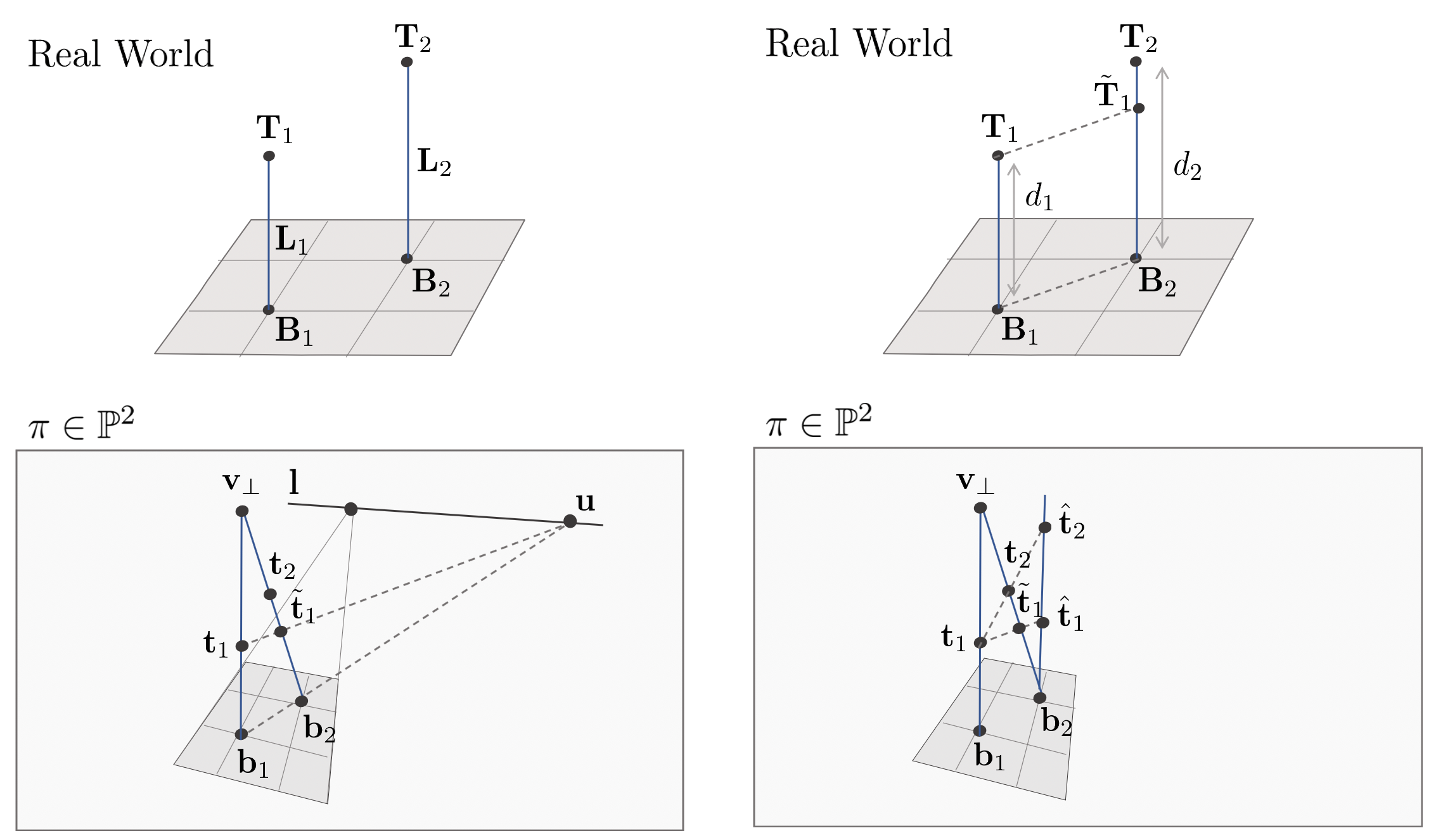
3차원 공간 상의 평면 $\pi$에 수직인 물체들의 소실점을 수직소실점(vertical vanishing point) $\mathbf{v_{\perp}}$라고 한다.
4.7.1. Result 8.24
평면 $\pi$의 소실선 $\mathbf{l}$과 수직소실점을 이용하면 물체의 크기를 스케일을 제외한 파라미터(up to scale)까지 계산할 수 있다. 정확하게 말하면 소실선 $\mathbf{l}$과 수직소실점 $\mathbf{v}_{\perp}$를 알면 평면 $\pi$에 수직한 선분들의 상대적 길이를 알 수 있다.
예를 들면, 3차원 공간 상의 평면 $\pi$에 위치한 두 점 $\mathbf{B}_{1}, \mathbf{B}_{2}$가 있고 이를 지나면서 $\pi$에 수직인 직선 $\mathbf{L}_{1}, \mathbf{L}_{2}$가 있다고 가정한다. 그리고 두 직선 $\mathbf{L}_{1}, \mathbf{L}_{2}$의 끝점 $\mathbf{T}_{1}, \mathbf{T}_{2}$가 있을 경우 소실선 $\mathbf{l}$과 수직소실점 $\mathbf{v}_{\perp}$를 사용하여 $\mathbf{T}_{1}, \mathbf{T}_{2}$의 상대적 길이를 측정할 수 있다.
우선, 모든 요소들을 이미지 평면에 프로젝션시킨다. 이 때, $\mathbf{b}_{1}, \mathbf{b}_{2}$를 잇는 직선과 소실선 $\mathbf{l}$이 만나는 점을 $\mathbf{u}$라고 정의한다. 그리고 $\mathbf{t}_{1}$에서 $\bar{\mathbf{b}_{1}\mathbf{b}_{2}}$에 평행한 직선을 그으면 해당 직선은 $\mathbf{u}$와 접한다. 이 때 $\bar{\mathbf{t}_{1}\mathbf{u}}$와 $\mathbf{v}_{\perp}\mathbf{b}_{2}$가 만나는 교점을 $\tilde{\mathbf{t}}_{1}$이라고 한다.
다음으로 $\bar{\mathbf{v}_{\perp}\mathbf{b}_{2}}$ 직선을 $\mathbb{P}^{1}$ 공간의 수직소실점 $\mathbf{v}_{\perp}$는 무한대의 점 $(1,0)$이 되고 $\mathbf{b}_{1}$은 원점 $(0,1)$되는 직선으로 프로젝션시킨다. 이 때 사용하는 Homography $\mathbf{H}_{2\times2}$는 다음과 같다.
\begin{equation}
\begin{aligned}
\mathbf{H}_{2\times2} = \begin{bmatrix} 1 & 0 \\ 1 & -\mathbf{v}_{\perp} \end{bmatrix}
\end{aligned}
\end{equation}
$\mathbf{H}_{2\times2}$는 Cross-Ratio를 보장한다. 다음으로 길이의 비를 이용하여 $d_{1} : d_{2} = \mathbf{b}_{1}\tilde{\mathbf{t}}_{1}:\mathbf{b}_{1}\mathbf{t}_{2}$의 비율을 구한다.
\begin{equation}
\begin{aligned}
\frac{d_{1}}{d_{2}} = \frac{\tilde{\mathbf{t}}_{1}(\mathbf{v}_{\perp}-\mathbf{t}_{2})}{\mathbf{t}_{2}(\mathbf{v}_{\perp}-\tilde{\mathbf{t}}_{1})}
\end{aligned}
\end{equation}
만약, 수직소실점 $\mathbf{v}_{\perp}$와 카메라의 주축(principal axis)이 수직인 경우 이미지 상에서 수직소실점은 만나지 않게 되고 아래와 같이 단순하게 비율을 계산할 수 있다.
\begin{equation}
\begin{aligned}
\frac{d_{1}}{d_{2}} = \frac{\tilde{\mathbf{t}}_{1}-\mathbf{b}_{2}}{\mathbf{t}_{2}-\mathbf{b}_{2}}
\end{aligned}
\end{equation}
4.8. Determining camera calibration $\mathbf{K}$ from a single view
단안 이미지에서 내부 파라미터 $\mathbf{K}$를 결정하기 위해서는 2가지 제약조건이 필요하다. 이미지 제약조건(scene constraint)과 내부 파라미터의 제약조건(internal constraint)이 있다.
이미지 제약조건으로는 이미지 평면에 존재하는 서로 수직인 두 소실점 $\mathbf{v}_{1}, \mathbf{v}_{2}$가 있을 경우 $\mathbf{v}_{1}^{\intercal}\mathbf{w}\mathbf{v}_{2}=0$가 있고, 소실선 $\mathbf{l}$과 소실점 $\mathbf{v}$가 직교하는 경우 이들의 Back-projection은 $\mathbf{l} = \mathbf{wx}$가 있다.
\begin{equation}
\begin{aligned}
& \mathbf{v}_{1}^{\intercal}\mathbf{w}\mathbf{v}_{2}=0 \\
& \mathbf{l} \times (\mathbf{wv}) = 0
\end{aligned}
\end{equation}
4.8.1. Result 8.26
내부 파라미터 제약조건으로는 $\mathbf{K}$가 Zero-Skew인 경우 $w_{12} = w_{21}=0$이 있고 또한, Square Pixels인 경우 $w_{12}=w_{21}=0, w_{11}=w_{22}$가 있다.
\begin{equation}
\begin{aligned}
& w_{12} = w_{21} \quad \text{for zero skew} \\
& w_{12}=w_{21}=0, w_{11}=w_{22} \quad \text{for square pixel}
\end{aligned}
\end{equation}
위와 같이 $\mathbf{w} = \begin{bmatrix} w_{1} & w_{2} & w_{4} \\ w_{2} & w_{3} &w_{5} \\ w_{4} & w_{5} & w_{6} \end{bmatrix}$ 파라미터를 찾기 위해 충분한 제약조건을 확보한 후 $\mathbf{w}$를 6차원 벡터로 정렬하여 $\mathbf{Ax}=0$ 형태의 선형 시스템을 만든다. 다음으로 특이값 분해(SVD)를 사용하여 $\mathbf{w}=\mathbf{K}^{-\intercal}\mathbf{K}^{-1}$ 값을 계산한 후 Cholesky Decomposition을 사용하여 $\mathbf{K}^{-\intercal}\mathbf{K}^{-1}$를 분해한다. 이를 통해 내부 파라미터 $\mathbf{K}$를 계산할 수 있다.
4.9. Calibration from three orthogonal vanishing points
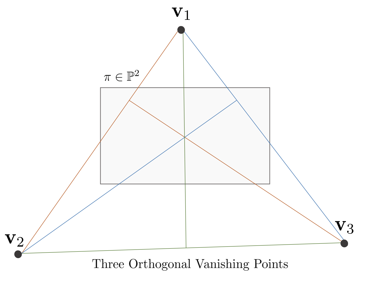
내부 파라미터 $\mathbf{K}$가 Zero-Skew이고 Square Pixel일 때 세 개의 서로 직교하는 수직소실점들 $\mathbf{v}_{i}, \ i=1,2,3$을 사용하여 $\mathbf{K}$를 계산할 수 있다. 우선 $\mathbf{K}$가 Zero-Skew이고 Square Pixel이므로 다음이 성립한다.
\begin{equation}
\begin{aligned}
\mathbf{w} = \begin{bmatrix} w_{1} & 0 & w_{2} \\ 0 & w_{1} & w_{3} \\ w_{2} & w_{3} & w_{4} \end{bmatrix}
\end{aligned}
\end{equation}
이와 같이 총 4개의 자유도를 가지므로 세 개의 수직소실점들을 사용하여 $\mathbf{K}$를 결정할 수 있다. 우선, 각각의 수직소실점들의 직교 특성을 사용하여 $\mathbf{v}_{i}^{\intercal}\mathbf{w}\mathbf{v}_{j}, \ \forall i\neq j$를 계산한다. 이 때 $\mathbf{w}$를 벡터화하여 $\mathbf{Ax}=0$ 형태의 선형 시스템으로 변환한 후 Nul $(\mathbf{A})$를 계산함으로써 $\mathbf{w}$를 구한다. 다음으로 Cholesky Decomposition을 사용하여 $\mathbf{w}=\mathbf{K}^{-\intercal}\mathbf{K}^{-1}$를 분해한다. 이와 같이 내부 파라미터 $\mathbf{K}$를 계산할 수 있다.
4.10. Computation of focal length and principal point using vanishing point and vanishing line
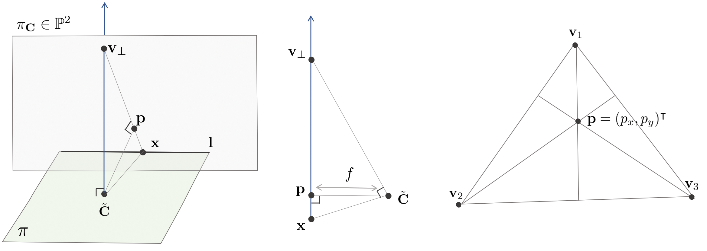
3차원 공간 상의 평면 $\pi$로부터 구할 수 있는 소실선 $\mathbf{l}$이 있고 $\pi$와 수직인 수직소실점 $\mathbf{v}_{\perp}$가 있다고 하면 이를 활용하여 초점거리 f와 주점(principal point)를 구할 수 있다.
초점거리 f를 구하는 방법은 다음과 같다. 수직소실점을 $\mathbf{v}_{\perp}$이라고 하고 이미지 평면 $\pi_{\mathbf{C}}$과 평면 $\pi$의 교차선을 $\mathbf{l}$이라고 하면 $\mathbf{v}_{\perp}\tilde{\mathbf{C}}$와 $\mathbf{x}\tilde{\mathbf{C}}$는 서로 직교한다. 그리고 카메라 중심에서 이미지 평면으로 수선을 내린 점 P가 있으면 $\tilde{\mathbf{C}}\mathbf{p}$의 길이가 곧 초점거리 f가 된다. $\mathbf{v}_{\perp}x$를 지름으로 하는 원을 그린 후 점 $\mathbf{p}$에 수평으로 그린 선과 원의 교점을 각각 $\mathbf{a}, \mathbf{b}$라고 하면 두 점 중 하나가 곧 카메라의 중심 $\tilde{\mathbf{C}}$가 되고 이는 곧 $\mathbf{ap} = \mathbf{bp}$가 초점거리 f가 된다.
주점(principal point) P를 구하는 방법은 다음과 같다. 수직소실점을 $\mathbf{v}_{1}$라고 하고 이미지 평면과 $\pi$ 평면의 교차선을 $\mathbf{l}_{1}$라고 하면 $\mathbf{v}_{1}$에서 $\mathbf{l}_{1}$에 수선을 내리면 해당 수선에 주점(principal point) $\mathbf{p}$가 위치한다. 이러한 특징으로 인해 서로 다른 세 개의 수직소실점이 존재하는 경우 이들의 수심(orthocenter of the triangle)이 곧 주점 $\mathbf{p}$가 된다.
4.11. The calibrating conic
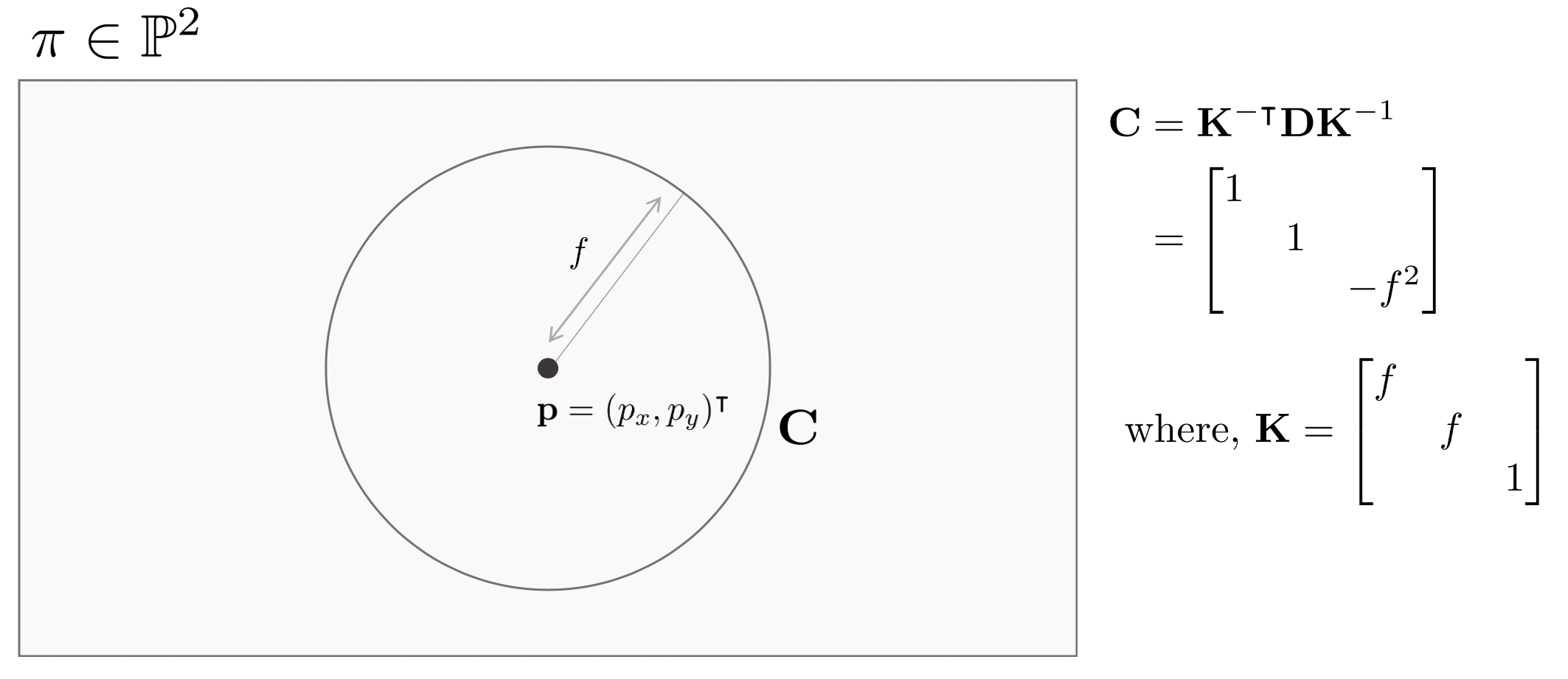
IAC(image of absolute conic)은 이미지 평면의 점을 Back-projection한 직선들 간의 각도를 구할 수 있고 Metric Rectification도 수행할 수 있는 유용한 도구이지만 Circular Point의 특성 상 실수의 근을 갖지 않아서 시각화가 불가능하다는 단점이 있다. 이를 보완하기 위해 고안된 것이 Calibration Conic이다. Calibration Conic은 $X^{2}+Y^{2}=Z^{2}$의 Cone을 프로젝션시킨 Image Conic을 의미하고 시각화가 가능한 장점이 존재한다.
카메라 프로젝션 $\mathbf{P} = \mathbf{K}[\mathbf{I}|0]$이 있을 때 Calibration Conic 위의 점들은 다음과 같이 프로젝션된다.
\begin{equation}
\begin{aligned}
\mathbf{C} = \mathbf{K}^{-\intercal}\begin{bmatrix} 1 & & \\ & 1 & \\ & & -1 \end{bmatrix}\mathbf{K}^{-1}
\end{aligned}
\end{equation}
이 때, $\mathbf{D}= \begin{bmatrix} 1 & & \\ & 1 & \\ & & -1 \end{bmatrix}$라고 하면 $\mathbf{C} = \mathbf{K}^{-\intercal}\mathbf{D}\mathbf{K}^{-1}$와 같이 나타낼 수 있다. 만약 $\mathbf{K} = \begin{bmatrix} f & & \\ & f & \\ & & 1 \end{bmatrix}$인 경우 Calibration Conic은
\begin{equation}
\begin{aligned}
\mathbf{C} = \begin{bmatrix} 1 & & \\ & 1 & \\ & & -f^{2} \end{bmatrix}
\end{aligned}
\end{equation}
으로 나타낼 수 있고 이 때, Calibration Conic은 원점이 주점(principal point)이면서 반지름이 초점거리 f인 이미지 상의 원을 의미한다.
$\mathbf{C}$를 분해하면 다음과 같이 다시 정의할 수 있다.
\begin{equation}
\begin{aligned}
& \mathbf{C} = \mathbf{K}^{-\intercal}\mathbf{DK}^{-1} = \mathbf{K}^{-\intercal}\mathbf{K}^{-1}\mathbf{KDK}^{-1} \\
& \mathbf{C} = \mathbf{w}\mathbf{S} \quad \text{where, } \mathbf{S} = \mathbf{KDK}^{-1}
\end{aligned}
\end{equation}
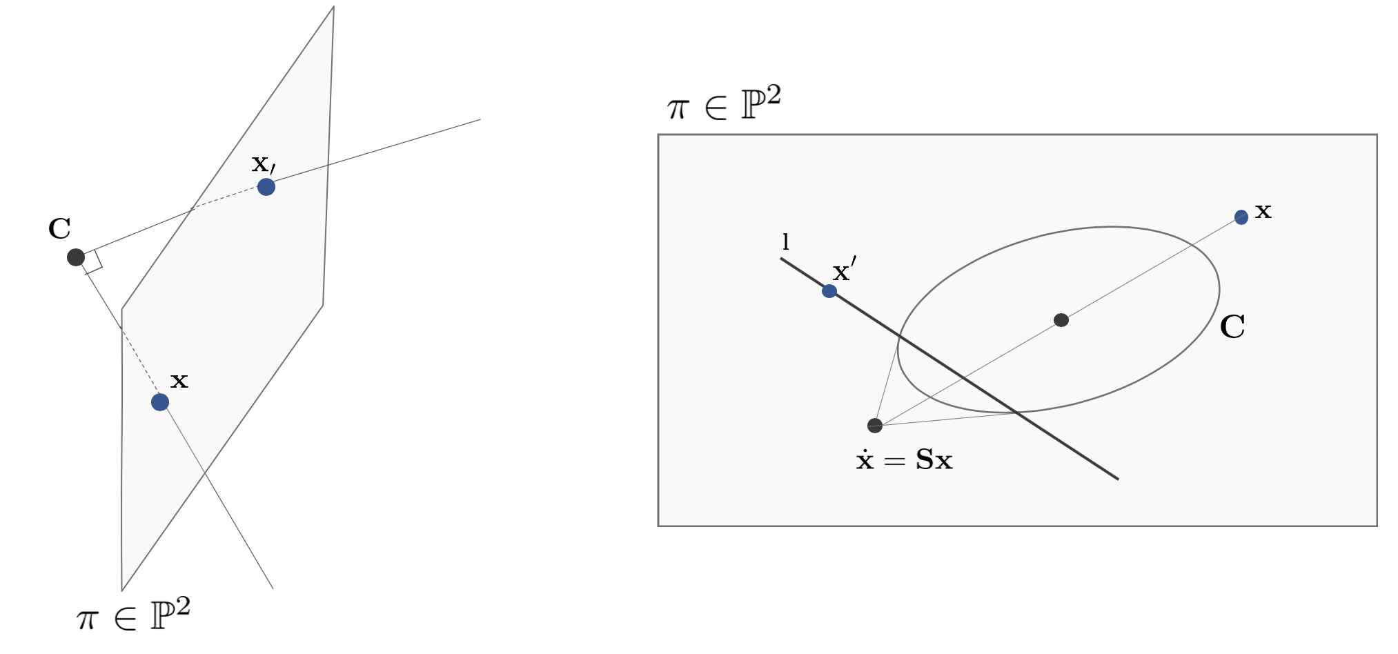
이 때 이미지 상의 임의의 점 $\mathbf{x}=\mathbf{K}\tilde{\mathbf{X}}$에 대하여 $\mathbf{Sx}$는 Calibration Conic에 의해 반사된 점(reflected point)을 의미한다.
\begin{equation}
\begin{aligned}
\mathbf{Sx} & = \mathbf{KDK}^{-1}\mathbf{K}\tilde{\mathbf{X}} \\
& = \mathbf{KD}\begin{bmatrix} X \\ Y \\ Z \end{bmatrix} = \mathbf{K}\begin{bmatrix} X \\ Y \\ -Z \end{bmatrix}
\end{aligned}
\end{equation}
이미지 평면 상의 두 점 $\mathbf{x}, \mathbf{x}^{\prime}$에 대하여 두 점의 Back-projection된 직선들이 서로 직교하는 경우 $\mathbf{x}^{\prime\intercal}\mathbf{wx}=0$이 성립한다. 이 식을 다시 작성하면
\begin{equation}
\begin{aligned}
& \mathbf{x}^{\prime\intercal}\mathbf{wx} = \mathbf{x}^{\prime\intercal}\mathbf{CS}^{-1}\mathbf{x} = \mathbf{x}^{\prime\intercal}\mathbf{CSx} = \mathbf{x}^{\prime\intercal}\mathbf{C}\dot{\mathbf{x}} \\
& \because \mathbf{S}^{-1} = \mathbf{S}
\end{aligned}
\end{equation}
이 때, $\dot{\mathbf{x}} = \mathbf{Sx}$는 점 $\mathbf{x}$가 Calibration Conic에 의해 반사된 점을 의미한다.
4.11.1. Result 8.30
결론적으로, 직선 $\mathbf{C}\dot{\mathbf{x}}$는 반사된 점 $\dot{\mathbf{x}}$와 Calibration Conic의 접선들을 이어주는 직선이 되고 점 $\mathbf{x}^{\prime}$는 직선 $\mathbf{C}\dot{\mathbf{x}}$ 위에 존재한다.
'Fundamental' 카테고리의 다른 글
| 다중관점기하학(Multiple View Geometry in Computer Vision) 책 내용 정리 Part 3 (0) | 2022.01.05 |
|---|---|
| 다중관점기하학(Multiple View Geometry in Computer Vision) 책 내용 정리 Part 2 (1) | 2022.01.05 |
| Plücker Coordinate 개념 정리 (3) | 2022.01.05 |
| 선형대수학 (Linear Algebra) 개념 정리 Part 1 (1) | 2022.01.05 |
| 리군 이론(Lie Theory) 개념 정리 - SO(3), SE(3) (9) | 2022.01.04 |


