 A L I D A
1. Introduction
로봇이 SLAM을 수행하는 동안 센서 데이터가 입력으로 들어오는데 순차적으로 들어오는 센서 데이터들의 차이를 통해 로봇의 포즈를 계산하는 알고리즘을 Odometry 또는 Front-end 라고 한다. 이 때, 센서 데이터의 노이즈로 인해 Odometry는 필연적으로 에러를 포함하고 있는데 시간이 지날수록 에러는 누적되어 전체적인 Trajectroy가 어긋나게 된다. 이러한 문제를 해결하기 위해 1997년 Lu and Milios는 로봇의 포즈를 그래프 자료구조로 표현함으로써 최적화하는 GraphSLAM 방법을 제안하였다.
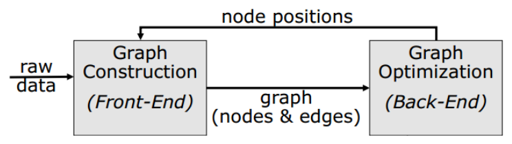
GraphSLAM의 Pipeline은 크게 Front-end와 Back-end로 구분할 수 있다. 로봇의 센서를 입력으로 받아 Pose Graph를 생성하는 부분을 Front-end라고 부르며 Front-end는 시간이 지날수록 노이즈로 인한 에러가 누적된다. 이렇게 누적된 에러를 최적화하는 부분을 Back-end라고 부르며 이 때 사용하는 알고리즘을 Pose Graph Optimization (PGO) 라고 한다. PGO는 로봇의 포즈만 변경시키고 맵 상에 존재하는 맵포인트들은 최적화하지 않는다. PGO와 달리 로봇의 포즈와 맵포인트를 동시에 최적화하는 방법을 Bundle Adjustment (BA)라고 한다. BA는 일반적으로 reprojection error를 에러함수로 설정하여 최적화를 수행하지만, PGO는 relative pose를 에러함수로 설정하여 최적화를 수행한다는 점이 다르다. 해당 포스트에서는 PGO만을 다룬다.
2. Pose graph
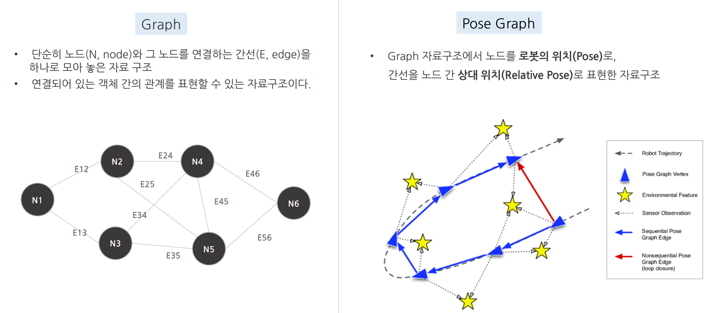
Pose Graph는 로봇의 포즈를 자료구조 중 하나인 그래프로 표현한 SLAM에 특화된 자료구조를 의미한다. Pose Graph에서 노드는 로봇의 포즈(Pose)로 나타내고 엣지는 노드 사이의 상대 포즈(Relative Pose)로 나타낸다. 아래 그림은 Graph와 Pose Graph 자료구조의 차이점을 나타낸 그림이다.
본 포스팅에서는 3차원 SLAM에 관한 내용을 다루므로 Pose Graph에서 Pose $\mathbf{x}$ 와 Edge $\mathbf{z}$ 는 다음과 같이 정의된다.
\begin{equation}
\begin{aligned}
\text{(Node) } \mathbf{x}_{i} & = [x_{i} \ \ y_{i} \ \ z_{i} \ \ \alpha_{i} \ \ \beta_{i} \ \ \gamma_{i}]^{\intercal} \\
\text{(Edge) } \mathbf{z}_{ij} & = [x_{ij} \ \ y_{ij} \ \ z_{ij} \ \ \alpha_{ij} \ \ \beta_{ij} \ \ \gamma_{ij}]^{\intercal} \\
\end{aligned}
\end{equation}
- $[x,y,z]$: 3차원 공간 상에서 로봇의 위치(position)
- $[\alpha, \beta, \gamma]$: 오일러 각도로 표현한 3차원 공간 상에서 로봇의 방향(orientation)
위 표현법은 로봇의 포즈를 위치와 오일러 각도(euler angle)로 기술한 표현법이다. 하지만, 대부분 SLAM 알고리즘의 경우 계산의 편의를 위해 변환 행렬(transformation matrix) 표현법을 사용한다.
\begin{equation}
\begin{aligned}
\text{(Node) } \mathbf{x}_{i} & = \begin{bmatrix} \mathbf{R}_{i} & \mathbf{t}_{i} \\ \mathbf{0}^{\intercal} & 1 \end{bmatrix} \in \mathbb{R}^{4\times 4} \\
\text{(Edge) } \mathbf{z}_{ij} & = \begin{bmatrix} \mathbf{R}_{ij} & \mathbf{t}_{ij} \\ \mathbf{0}^{\intercal} & 1 \end{bmatrix} \in \mathbb{R}^{4\times 4}
\end{aligned}
\end{equation}
- $\mathbf{R} \in \mathbb{R}^{3\times 3}$: 3차원 공간 상의 회전 행렬
- $\mathbf{t} = [t_x, t_y, t_z]^{\intercal}$: 3차원 공간 상의 병진 이동(translation)
이 때, $\mathbf{x}_{i}$는 i번째 포즈를 의미하며 $\mathbf{z}_{ij}$는 노드 i,j 사이의 상대포즈를 의미한다.
3. Pose graph optimization
3.1. Overall process
로봇이 이동하면서 front-end에 의해 pose graph를 생성하다가 같은 장소를 재방문하는 경우 loop detection 알고리즘이 동작하여 루프인지 여부를 판별한다. 이 때 루프가 탐지되면 기존 노드 $\mathbf{x}_{i}$와 재방문하여 생성된 노드 $\mathbf{x}_{j}$가 loop edge로 연결되고 back-end에서 PGO를 수행한다.
PGO가 수행되는 과정을 단계별로 정리하면 다음과 같다.
- front-end에 의해 포즈를 계산한 후 pose graph를 순차적으로 생성
- 로봇이 같은 장소를 재방문하면 loop detection 알고리즘이 작동
- 루프가 탐지되면 기존 노드 $\mathbf{x}_{i}$와 새로운 노드 $\mathbf{x}_{j}$ 사이에 loop edge가 생성됨
- loop edge로 연결된 두 노드의 상대포즈를 예측값으로 설정하고 두 노드의 센서 데이터를 매칭하여 관측값을 생성함. 이 때, 비순차적인 노드의 관측값은 실제로 측정한 정보가 아니므로 virtual measurement라고 한다.
- back-end에서 관측값과 예측값의 차이, 즉 relative pose 에러가 최소가 되는 방향으로 에러함수를 최적화한다
3.2. Relative pose error derivation
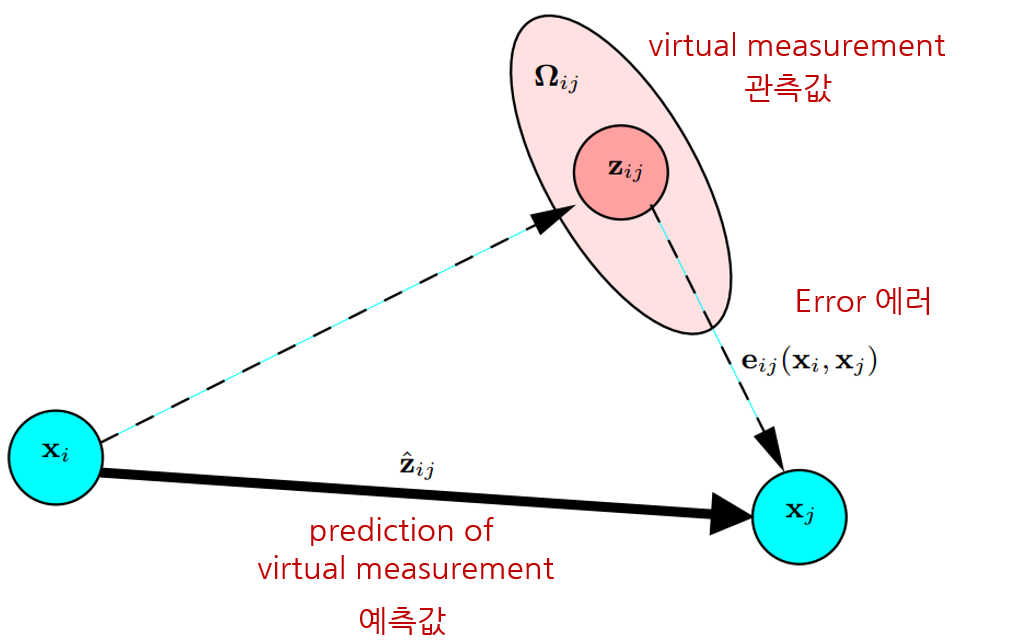
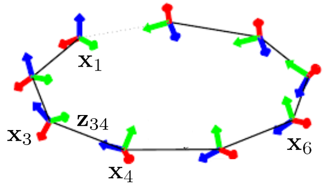
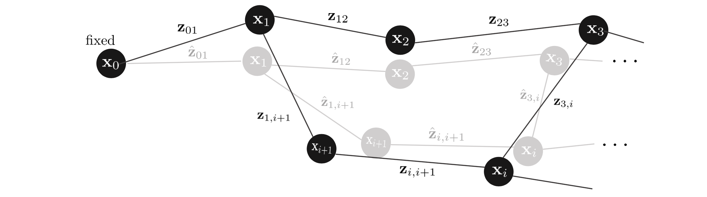
Pose graph 상에서 두 노드 $\mathbf{x}_{i}, \mathbf{x}_{j}$가 주어졌을 때 센서 데이터에 의해 새롭게 계산한 상대포즈(관측값) $\mathbf{z}_{ij}$와 기존의 알고 있는 상대포즈(예측값) $\hat{\mathbf{z}}_{ij}$의 차이를 relative pose 에러로 정의한다. (Freiburg univ. Robot Mapping Course 그림 참조).
\begin{equation}
\begin{aligned}
\mathbf{e}_{ij}(\mathbf{x}_{i},\mathbf{x}_{j}) = \mathbf{z}_{ij}^{-1}\hat{\mathbf{z}}_{ij} = \mathbf{z}_{ij}^{-1} \mathbf{x}_{i}^{-1}\mathbf{x}_{j}
\end{aligned}
\end{equation}
relative pose 에러를 최적화하는 과정을 pose graph optimization(PGO)라고 하며 graph-based SLAM의 back-end 알고리즘으로도 불린다. Front-end의 visual odometry(VO) 또는 lidar odometry(LO)에 의해 순차적으로 계산되는 노드 $\mathbf{x}_{i}, \mathbf{x}_{i+1}, \cdots$는 관측값과 예측값이 동일하기 때문에 PGO가 수행되지 않지만 loop closing이 발생하여 비순차적인 두 노드 $\mathbf{x}_{i}, \mathbf{x}_{j}$ 사이에 엣지가 연결되면 관측값과 예측값의 차이가 발생하기 때문에 PGO가 수행된다.
즉, PGO는 일반적으로 loop closing과 같은 특수한 상황이 발생할 때 수행된다. 로봇이 이동하면서 같은 장소를 재방문하는 경우 loop detection 알고리즘이 동작하여 루프인지 여부를 판별한다. 이 때 루프가 탐지되면 기존 노드 $\mathbf{x}_{i}$와 재방문하여 생성된 노드 $\mathbf{x}_{j}$가 loop edge로 연결되고 여러 매칭 알고리즘 (GICP, NDT, etc...)에 의해 관측값을 생성한다. 이러한 관측값은 실제로 관측한 값이 아닌 매칭 알고리즘에 의해 생성된 가상의 관측값이므로 virtual measurement라고 불린다.
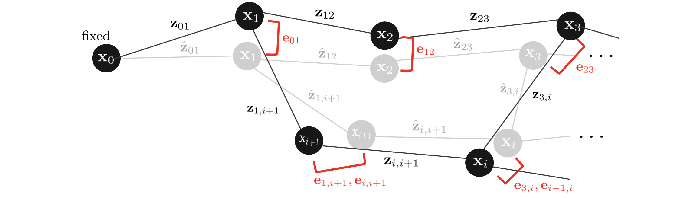
Pose graph 상의 모든 노드에 대한 relative pose 에러는 다음과 같이 정의할 수 있다.
\begin{equation}
\begin{aligned}
\mathbf{E}(\mathbf{x}) & = \arg\min_{\mathbf{x}^{*}} \sum_{i}\sum_{j} \left\| \mathbf{e}_{ij} \right\|^{2} \\
& = \arg\min_{\mathbf{x}^{*}} \sum_{i}\sum_{j} \mathbf{e}_{ij}^{\intercal}\mathbf{e}_{ij}
\end{aligned}
\end{equation}
$\mathbf{E}(\mathbf{x}^{*})$를 만족하는 $\left\|\mathbf{e}(\mathbf{x}^{*})\right\|^{2}$를 non-linear least squares를 통해 반복적으로 계산할 수 있다. 작은 증분량 $\Delta \mathbf{x}$를 반복적으로 $\mathbf{x}$에 업데이트함으로써 최적의 상태를 찾는다.
\begin{equation}
\begin{aligned}
\mathbf{E}(\mathbf{x} + \Delta \mathbf{x}) & = \arg\min_{\mathbf{x}^{*}} \sum_{i}\sum_{j} \left\|\mathbf{e}_{ij}(\mathbf{x}_{i} + \Delta \mathbf{x}_{i},\mathbf{x}_{j} + \Delta \mathbf{x}_{j})\right\|^{2}
\end{aligned}
\end{equation}
엄밀하게 말하면 상태 증분량 $\Delta \mathbf{x}$은 SE(3) 변환행렬이므로 $\oplus$ 연산자를 통해 기존 상태 $\mathbf{x}$에 더해지는게 맞지만 표현의 편의를 위해 $+$ 연산자를 사용하였다.
\begin{equation}
\begin{aligned}
\mathbf{e}_{ij}(\mathbf{x}_{i} \oplus \Delta \mathbf{x}_{i},\mathbf{x}_{j} \oplus \Delta \mathbf{x}_{j})
\quad \rightarrow \quad\mathbf{e}_{ij}(\mathbf{x}_{i} + \Delta \mathbf{x}_{i},\mathbf{x}_{j} + \Delta \mathbf{x}_{j})
\end{aligned}
\end{equation}
위 식은 테일러 1차 근사를 통해 다음과 같이 표현이 가능하다.
\begin{equation}
\begin{aligned}
\mathbf{e}_{ij}(\mathbf{x}_{i} + \Delta \mathbf{x}_{i},\mathbf{x}_{j} + \Delta \mathbf{x}_{j}) & \approx \mathbf{e}_{ij}(\mathbf{x}_{i} ,\mathbf{x}_{j} ) + \mathbf{J}_{ij} \begin{bmatrix} \Delta \mathbf{x}_{i} \\ \Delta \mathbf{x}_{j} \end{bmatrix} \\ & = \mathbf{e}_{ij}(\mathbf{x}_{i} ,\mathbf{x}_{j} ) + \mathbf{J}_{i}\Delta \mathbf{x}_{i} + \mathbf{J}_{j}\Delta \mathbf{x}_{j} \\
& = \mathbf{e}_{ij}(\mathbf{x}_{i} ,\mathbf{x}_{j} ) + \frac{\partial \mathbf{e}_{ij}}{\partial \mathbf{x}_{i}} \Delta \mathbf{x}_{i} + + \frac{\partial \mathbf{e}_{ij}}{\partial \mathbf{x}_{j}} \Delta \mathbf{x}_{j}
\end{aligned} \label{eq:rel14}
\end{equation}
\begin{equation}
\begin{aligned}
\mathbf{E}(\mathbf{x} + \Delta \mathbf{x}) & \approx \arg\min_{\mathbf{x}^{*}} \sum_{i}\sum_{j} \left\|\mathbf{e}_{ij}(\mathbf{x}_{i}, \mathbf{x}_{j}) + \mathbf{J}_{ij} \begin{bmatrix} \Delta \mathbf{x}_{i} \\ \Delta \mathbf{x}_{j} \end{bmatrix} \right\|^{2} \\
\end{aligned}
\end{equation}
이를 미분하여 모든 노드에 대한 최적의 증분량 $\Delta \mathbf{x}^{*}$ 값을 구하면 다음과 같다. 자세한 유도 과정은 본 섹션에서는 생략한다. 유도 과정에 대해 자세히 알고 싶으면 [SLAM] Errors and Jacobian Derivations for SLAM 정리 포스트를 참조하면 된다.
\begin{equation}
\begin{aligned}
& \mathbf{J}^{\intercal}\mathbf{J} \Delta \mathbf{x}^{*} = -\mathbf{J}^{\intercal}\mathbf{e} \\
& \mathbf{H}\Delta \mathbf{x}^{*} = - \mathbf{b} \\
\end{aligned} \label{eq:rel6}
\end{equation}
위 식은 선형시스템 $\mathbf{Ax} = \mathbf{b}$ 형태이므로 schur complement, cholesky decomposition과 같은 다양한 선형대수학 테크닉을 사용하여 $\Delta \mathbf{x}^{*}$를 구할 수 있다. 이렇게 구한 최적의 증분량을 현재 상태에 더한다. 이 때, 기존 상태 $\mathbf{x}$의 오른쪽에 곱하느냐 왼쪽에 곱하느냐에 따라서 각각 로컬 좌표계에서 본 포즈를 업데이트할 것 인지(오른쪽) 전역 좌표계에서 본 포즈를 업데이트할 것 인지(왼쪽) 달라지게 된다. relative pose 에러는 두 노드의 상대 포즈에 관련되어 있으므로 로컬 좌표계에서 업데이트하는 오른쪽 곱셈이 적용된다.
\begin{equation}
\begin{aligned}
\mathbf{x} \leftarrow \mathbf{x} \oplus \Delta \mathbf{x}^{*}
\end{aligned}
\end{equation}
오른쪽 곱셈 $\oplus$ 연산의 정의는 다음과 같다.
\begin{equation}
\begin{aligned}
\mathbf{x} \oplus \Delta \mathbf{x}^{*}& = \mathbf{x} \Delta \mathbf{x}^{*} \\& = \mathbf{x} \exp([\Delta \xi^{*}]_{\times}) \quad \cdots \text{ locally updated (right mult)} \end{aligned} \label{eq:rel2}
\end{equation}
3.2.1. Jacobian of relative pose error
Relative pose 에러의 SE(3) 버전 자코비안은 다음과 같다.
\begin{equation}
\boxed{ \begin{aligned}
& \frac{\partial \mathbf{e}_{ij} }{\partial \Delta \xi_{i}} = -\mathcal{J}^{-1}_{r}\text{Ad}_{\mathbf{x}_{j}^{-1}} \in \mathbb{R}^{6\times6} \\
& \frac{\partial \mathbf{e}_{ij} }{\partial \Delta \xi_{j}} = \mathcal{J}^{-1}_{r}\text{Ad}_{\mathbf{x}_{j}^{-1}} \in \mathbb{R}^{6\times6}
\end{aligned} }
\end{equation}
자세한 유도 과정은 [SLAM] Errors and Jacobian Derivations for SLAM 정리 포스트의 내용을 참조하면 된다.
3.3. Graphical explanation of PGO
PGO의 과정을 그림으로 순차적으로 나타내면 다음과 같다. 자율주행차량이 주행을 하면서 PGO + Loop Closing이 발생하는 상황을 예로 들어서 설명해본다. 해당 시나리오는 LiDAR SLAM 알고리즘 중 하나인 HDL Graph SLAM 코드를 참고하여 작성하였다.
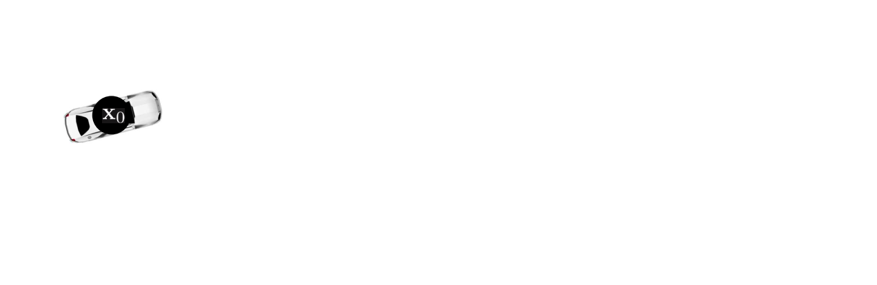
[1] 차량이 주행을 시작하면 가장 첫번째 키프레임을 노드 $\mathbf{x}_{0}$로 추가한다. 노드 $\mathbf{x}_{i}$는 $i$번 째 키프레임을 의미하며 pose graph의 노드이므로 포즈 $\mathbf{T}_{i}$의 정보를 포함한다.
\begin{equation}
\begin{aligned}
\mathbf{x}_{i} = \mathbf{T}_{i} = \begin{bmatrix} \mathbf{R}_{i} & \mathbf{t}_{i} \\ \mathbf{0} & 1 \end{bmatrix}
\end{aligned}
\end{equation}
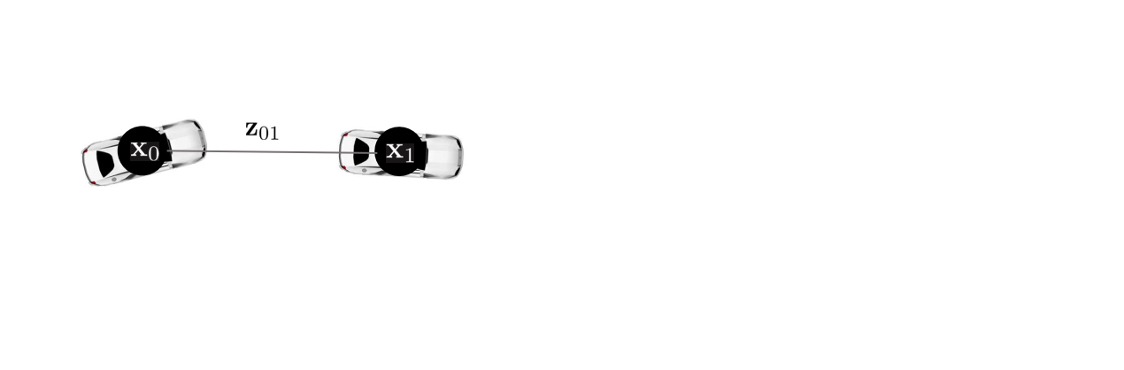
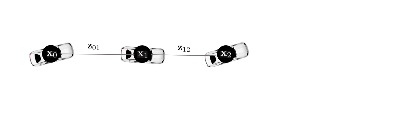
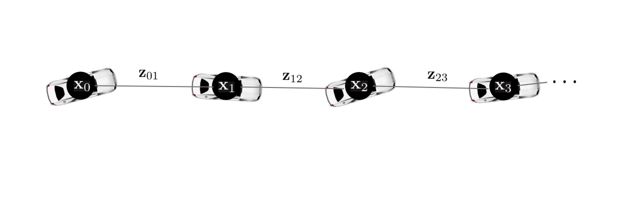
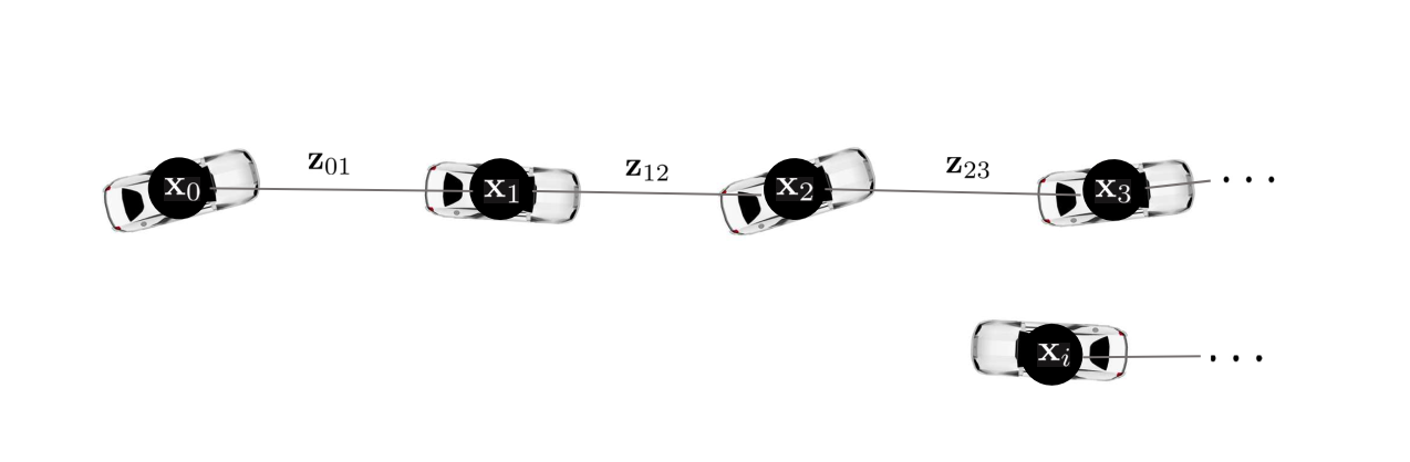
[2] 다음으로 front-end에 의해 순차적으로 차량의 포즈를 계산한다. HDL Graph SLAM에서는 포즈를 계산하기 위해 LiDAR 스캔 매칭 알고리즘(e.g., GICP, NDT)이 사용되었다.
- front-end에서 스캔 매칭 알고리즘을 활용하여 새로운 포즈를 계산한다.
- 새로운 포즈가 $\mathbf{x}_{0}$ 노드로부터 일정 거리 이상 멀어지면 $\mathbf{x}_{1}$ 노드를 생성하여 pose graph에 추가한다.
- 두 노드 사이의 상대포즈 $\mathbf{z}_{01}$을 계산하여 엣지에 추가한다.
순차적으로 추가되는 노드들은 관측값(measurement)와 예측값이 동일하므로 PGO를 수행해도 포즈 업데이트가 발생하지 않는다. 자율주행차량이 동일한 장소를 방문하여 loop edge가 생성되기 전까지 pose graph에 노드를 추가한다.
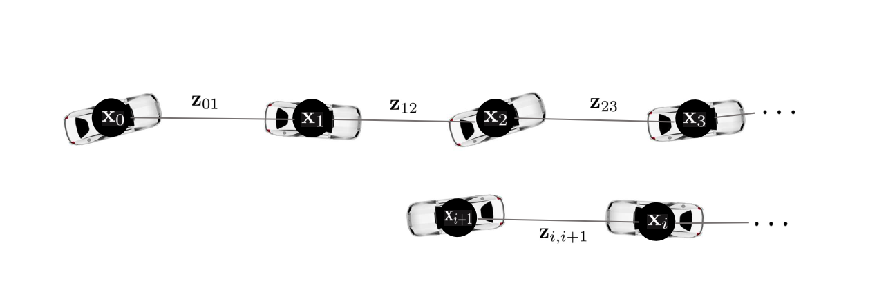
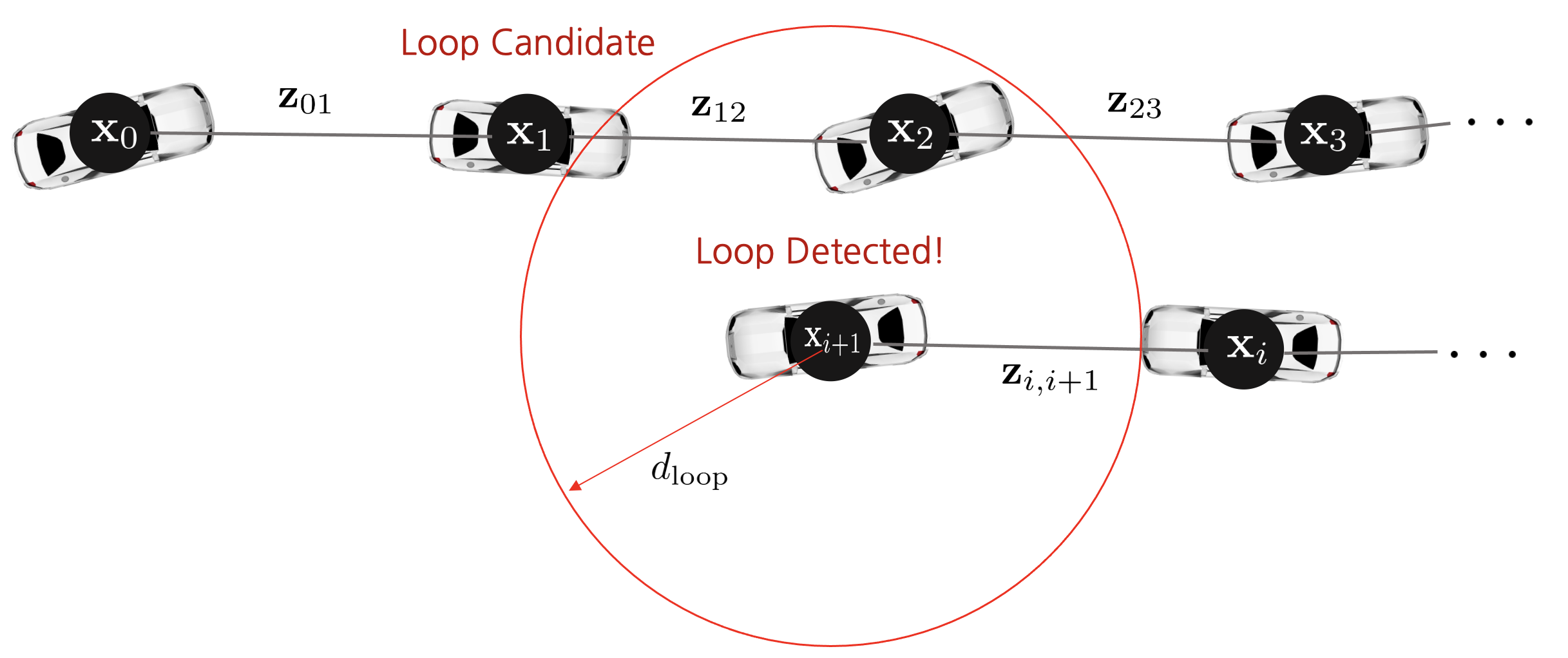
[3] 자율주행차량이 이전 pose graph 노드들과 근접한 장소에 위치하면 loop detection 알고리즘을 수행하여 루프를 탐지한다. HDL Graph SLAM의 경우 거리를 기반으로 루프를 탐지한다.
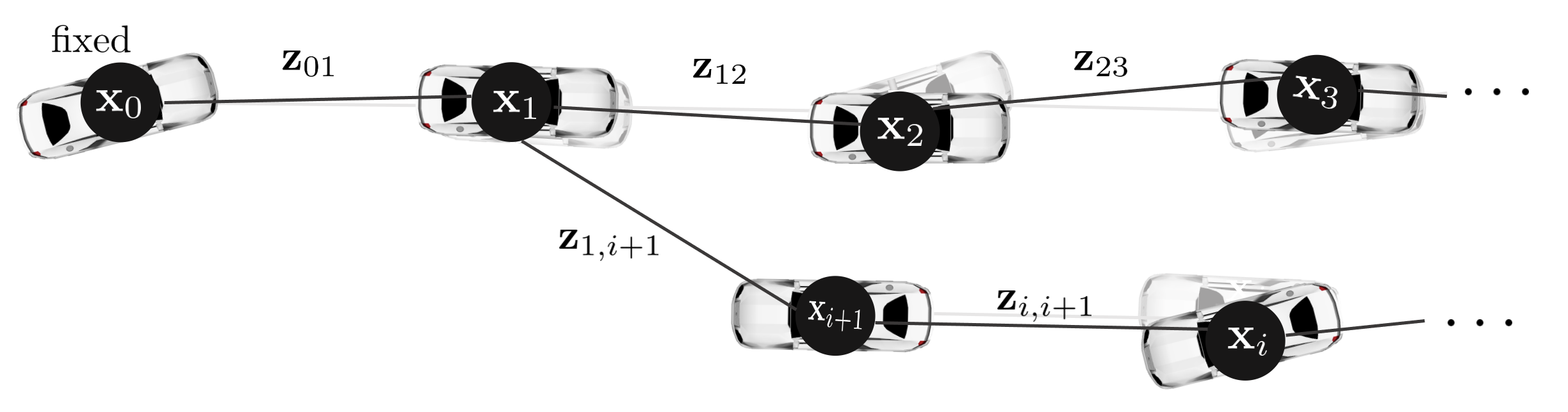
[4] 다음으로 loop edge를 연결할 후보군을 찾아야 한다. $\mathbf{x}_{i+1}$ 노드에서 loop detection 알고리즘를 수행하여 $\mathbf{x}_{1}$ 노드와 루프를 탐지했다고 가정하자. 루프가 발견되면 가장 처음 발견된 노드 $\mathbf{x}_{1}$를 후보(candidate) 루프 노드로 등록한다.
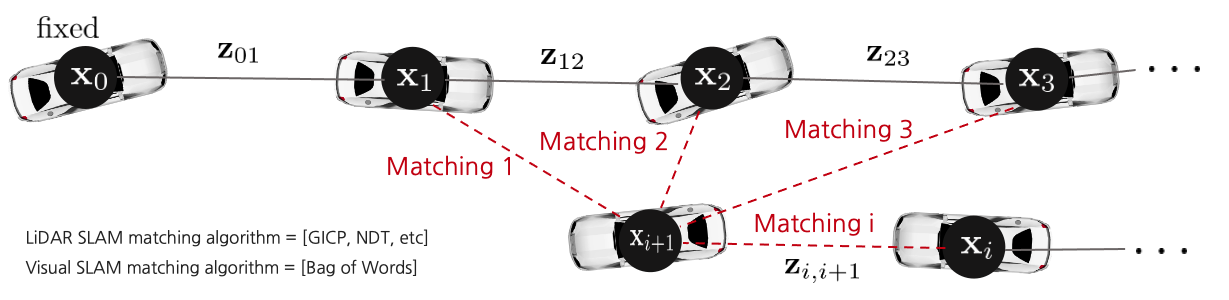
[5] $\mathbf{x}_{i+1}$와 후보 루프 노드 $\mathbf{x}_{1}$부터 순차적으로 센서 데이터를 매칭하여 노드의 매칭 점수를 각각 계산한다$(\mathbf{x}_{1} \sim \mathbf{x}_{i})$. 이 때, front-end와 동일한 스캔 매칭 알고리즘 (e.g., GICP, NDT)을 사용하였다. HDL Graph SLAM에서 $\mathbf{x}_{i}$ 노드의 센서 데이터는 $\mathcal{P}_{i}$는 LiDAR 포인트클라우드를 의미한다.
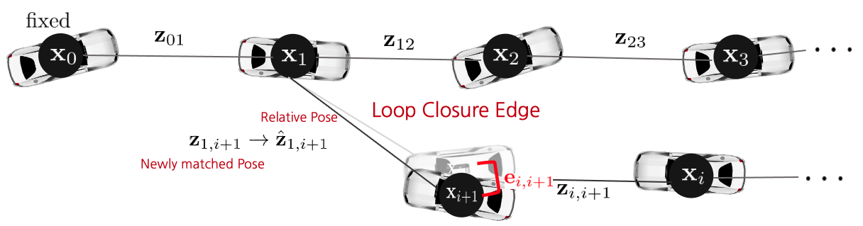
[6] 스캔 매칭 점수가 가장 높은 노드 (예시에서는 $\mathbf{x}_{1}$ 노드)와 loop closure edge를 생성하고 스캔 매칭으로 계산된 포즈 값을 관측값(virtual measurement) $\mathbf{z}_{1,i+1}$으로 설정하고, 두 노드 x_1, x_i+1의 상대포즈를 예측값 $\hat{\mathbf{z}}_{1,i+1}$으로 설정한다.
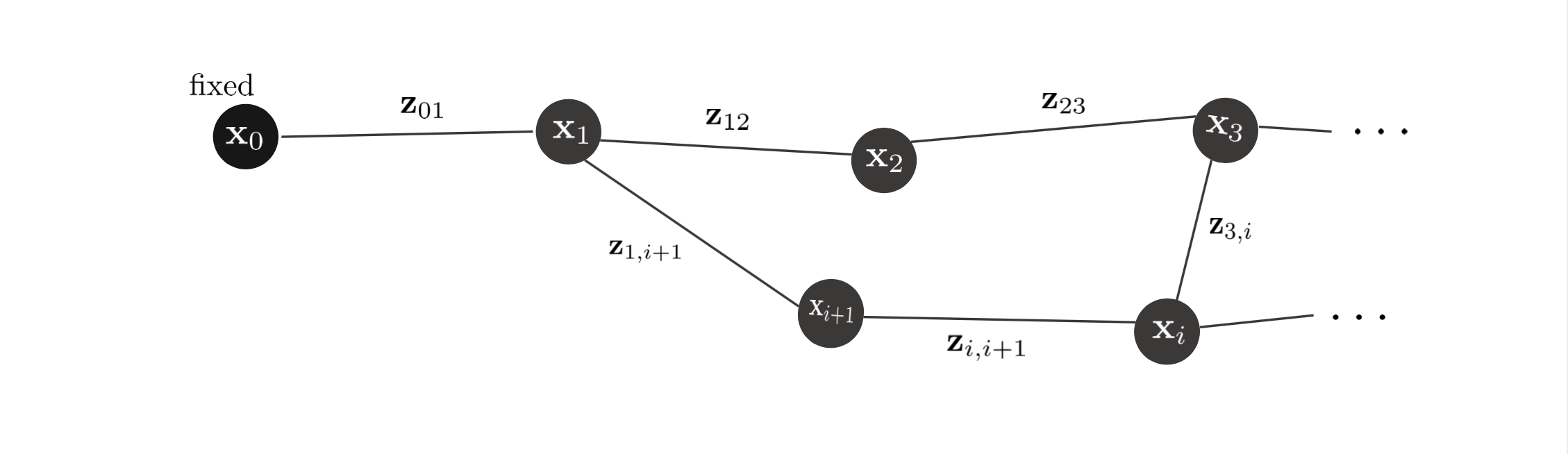
[7] back-end에서 PGO를 수행하여 관측값과 예측값의 차이인 relative pose 에러가 최소화되는 차량의 포즈 증분량 $\Delta \mathbf{x}^{*}$를 계산한다. 이 때 비선형 최소제곱법(e.g., GN, LM)을 통해 반복적으로 relative pose 에러가 최소가 되는 차량의 포즈를 업데이트한다.
\begin{equation}
\begin{aligned}
\mathbf{e}_{ij}(\mathbf{x}_{i},\mathbf{x}_{j}) = \mathbf{z}_{ij}^{-1}\hat{\mathbf{z}}_{ij} = \mathbf{z}_{ij}^{-1} \mathbf{x}_{i}^{-1}\mathbf{x}_{j}
\end{aligned}
\end{equation}
\begin{equation*}
\begin{aligned}
& \text{optimize all i,j nodes in the pose graph} \\
\end{aligned}
\end{equation*}
\begin{equation}
\begin{aligned}
& \mathbf{x}_{i} \leftarrow \mathbf{x}_{i} \oplus \Delta \mathbf{x}_{i}^{*} \\ & \mathbf{x}_{j} \leftarrow \mathbf{x}_{j} \oplus \Delta \mathbf{x}_{j}^{*} \\
\end{aligned}
\end{equation}
4. Example code review
PGO를 테스트해 볼 수 있는 예제 코드를 작성하였다. 코드는 링크를 통해 다운로드 및 실행 가능하다. 최적화 라이브러리로 g2o를 사용하였으며 ROS 환경에서 구동할 수 있도록 설정하였다. 보다 자세한 실행 방법은 링크 내에 설명되어 있다.
예제는 각 케이스마다 20번씩 최적화를 수행하며 20번이 지난 후에는 랜덤하게 초기화되어 다음 케이스로 넘어간다. 예제를 실행한 결과는 다음과 같다.
예제의 상황은 Front-end에서 Loop Closing이 발생한 상황부터 시작한다. 실제 Loop Closing에서는 Loop Closure Edge가 연결된 노드만 관측값이 변한 상태로 PGO가 수행되지만 본 예제에서는 모든 노드에 관측값을 랜덤하게 위치시킴으로써 에러가 감소하는 모습을 시각적으로 볼 수 있도록 하였다.
Loop Closing이 발생하면 Front-end에서 GICP를 통해 새로운 관측값 $\mathbf{z}_{ij}$를 구하고 기존의 값들은 예측값 $\hat{\mathbf{z}}_{ij}$으로 전환된다. 다음으로 관측값과 예측값을 Back-end로 전달한다.
Back-end에서 관측값과 예측값의 차이를 $\mathbf{e}_{ij}$로 설정하여 이전 섹션에서 설명한 GN, LM과 같은 방법을 통해 20번씩 최적화를 수행한다. 실제 SLAM 알고리즘에서 20번 최적화는 순식간에 완료되지만 시각화를 위해 천천히 최적화하도록 코드를 작성하였다.
4.1. Code
PGOToyExample::PGOToyExample(bool verbose)
    : vertex_id_(0), verbose_(verbose)
{
  num_poses_ = 15; // Pose 노드의 개수를 임의로 15개로 설정

  // g2o solve 설정 코드
  // Linear Solver는 Pose(6), Landmark(3)의 문제를 풀 때 사용하는 BlockSolver 설정
  // Optimizer는 Levenberg-Marquardt 방법 사용, Lambda 초기값 설정
  std::unique_ptr<g2o::BlockSolver_6_3::LinearSolverType> linear_solver;
  linear_solver = g2o::make_unique<g2o::LinearSolverDense<g2o::BlockSolver_6_3::PoseMatrixType>>();
  g2o::OptimizationAlgorithmLevenberg* solver =
      new g2o::OptimizationAlgorithmLevenberg(g2o::make_unique<g2o::BlockSolver_6_3>(std::move(linear_solver)));
  solver->setUserLambdaInit(1);
  optimizer_ = new g2o::SparseOptimizer();
  optimizer_->setAlgorithm(solver);
}
// 노이즈가 추가되기 전 초기 Pose 노드들을 생성하는 함수
void PGOToyExample::SetOriginalPoses() {
  for(int i=0; i<num_poses_; i++){
    // num+poses의 크기만큼 루프를 돌면서 각 노드마다 랜덤으로 노드의 초기 위치를 결정한다.
    // 0번 노드는 (0,0,0)으로 설정하고 7번 노드까지 직선으로 간다음 8번노드에서 옆으로 한 번 꺽고 9번부터 마지막 노드까지는 다시 원점으로 돌아오도록 설정하여 Loop Closing 형태의 노드가 되도록 설정한다.
    // 회전은 초기 노드들의 경우 Identity로 설정한다.
    Vec3 trans;
    if(i==0) {
      trans = Vec3(0,0,0);
    }
    else if(i>=1 && i <=7) {
      trans = Vec3(i + Sampling::Gaussian(.2),
                   Sampling::Gaussian(.2),
                   Sampling::Gaussian(.2));
    }
    else if(i==8) {
      trans = Vec3(8 + Sampling::Gaussian(.2),
                   7 - i + Sampling::Gaussian(.2),
                   Sampling::Gaussian(.2));
    }
    else if(i>=9) {
      trans = Vec3(17 - i + Sampling::Gaussian(.2),
                   -1 + Sampling::Gaussian(.2),
                   Sampling::Gaussian(.2));
    }

    Quaternion q;
    q.setIdentity();

    // g2o::SE3Quat 자료구조에 초기 pose들을 넣고 original_poses 벡터에 추가한다.
    g2o::SE3Quat pose;
    pose.setRotation(q);
    pose.setTranslation(trans);

    original_poses_.push_back(pose);
  }
}
// 초기 Pose 노드들에 노이즈를 추가한 후 해당 노드들을 g2o optimizer에 추가하는 함수
void PGOToyExample::MakeCurrentPoseAndAddVertex() {
  for(int i=0;i<original_poses_.size();i++){
    // original_poses 벡터의 크기만큼 루프를 돌면서 g2o optimizer에 추가할 g2o::VertexSE3Expmap 노드를 생성한다
    g2o::VertexSE3Expmap* vtx = new g2o::VertexSE3Expmap();
    vtx->setId(vertex_id_);

    // 첫번째 노드인 경우 해당 노드(또는 vertex)의 포즈를 고정시킨다.
    if(i==0){
      vtx->setFixed(true);
    }

    // 위치 노이즈를 랜덤 가우시안 샘플링으로 생성한다.
    // 회전에 관한 노이즈는 랜덤으로 생성한다.
    Vec3 trans(Sampling::Gaussian(.2),
               Sampling::Gaussian(.2),
               Sampling::Gaussian(.2));
    Quaternion q;
    q.UnitRandom();

    // 기존의 original_poses에 노이즈를 추가한 후 g2o optimizer에 노드로 추가한다
    // 이 때, 노드는 GICP에 의해 업데이트된 관측값으로 간주한다
    // 예측값은 엣지를 추가하는 코드에서 g2o optimizer에 추가된다
    g2o::SE3Quat origin = original_poses_.at(i);
    g2o::SE3Quat noise;
    noise.setTranslation(origin.translation() + trans);

    vtx->setEstimate(noise);
    optimizer_->addVertex(vtx);
    vertex_id_ += 1;
  }
}
// g2o optimizer에 엣지를 추가하는 함수
void PGOToyExample::AddEdge() {
  // 시간순으로(temporal) 생성된 엣지들을 g2o optimizer에 추가한다.
  for(int i=1;i<original_poses_.size();i++){
    g2o::EdgeSE3Expmap* e(new g2o::EdgeSE3Expmap());
    g2o::SE3Quat relative_pose = original_poses_.at(i-1).inverse() * original_poses_.at(i);
    e->setMeasurement(relative_pose);

    // Information matrix를 랜덤하게 생성한 후 g2o optimizer에 추가한다
    // 랜덤한 Information matrix의 영향으로 인해 에러의 반영율이 달라지게 된다
    MatXX A = Eigen::MatrixXd::Random(6,6).cwiseAbs();
    MatXX information = A.transpose() * A;
    e->setInformation(information);

    // g2o 노드들을 설정한 후 optimizer에 엣지를 추가한다
    e->vertices()[0] = optimizer_->vertex(i-1);
    e->vertices()[1] = optimizer_->vertex(i);

    // Add the edge into the g2o optimizer.
    optimizer_->addEdge(e);
  }

  // (5,11), (3,14)와 같이 비순차적으로(non-temporal) 연결된 Loop Closer 엣지들도 위와 같은 방법으로 추가한다
  g2o::EdgeSE3Expmap* e511(new g2o::EdgeSE3Expmap());
  g2o::SE3Quat relative_pose = original_poses_.at(5).inverse() * original_poses_.at(11);
  e511->setMeasurement(relative_pose);
  MatXX A = Eigen::MatrixXd::Random(6,6).cwiseAbs();
  MatXX information = A.transpose() * A;
  e511->setInformation(information);
  e511->vertices()[0] = optimizer_->vertex(5);
  e511->vertices()[1] = optimizer_->vertex(11);
  optimizer_->addEdge(e511);

  g2o::EdgeSE3Expmap* e314(new g2o::EdgeSE3Expmap());
  relative_pose = original_poses_.at(3).inverse() * original_poses_.at(14);
  e314->setMeasurement(relative_pose);
  A = Eigen::MatrixXd::Random(6,6).cwiseAbs();
  information = A.transpose() * A;
  e314->setInformation(information);
  e314->vertices()[0] = optimizer_->vertex(3);
  e314->vertices()[1] = optimizer_->vertex(14);
  optimizer_->addEdge(e314);
// 20번의 최적화가 끝난 후 다시 시작하기 위해 초기화하는 함수
void PGOToyExample::Reset() {
  // g2o optimizer의 모든 노드와 엣지의 정보를 초기화한다
  // 초기 Pose들도 제거하고 vertex_id 또한 0으로 초기화한다
  optimizer_->clear();
  original_poses_.clear();
  vertex_id_ = 0;

  // 초기 Pose들을 랜덤하게 다시 생성한다
  SetOriginalPoses();

  // 초기 Pose들에 노이즈를 추가한 후 g2o optimizer에 추가한다
  MakeCurrentPoseAndAddVertex();

  // g2o optimizer에 엣지를 다시 추가한다.
  AddEdge();

  // 최적화를 위해 optimizer 설정을 초기화한다
  // 최적화 과정을 프린트할지(verbose) 설정한다
  optimizer_->initializeOptimization();
  optimizer_->setVerbose(verbose_);
}
// PGOToyExample 객체를 생성한 후 ROS를 통해 시각화를 수행하는 함수
int main(int argc, char **argv) {
  // ros의 노드 이름 설정 및 NodeHandler 객체 생성
  ros::init(argc,argv,"pgo_toy_example");
  ros::NodeHandle nh, priv_nh("~");

  // Visualization을 수행하기 위한 다양한 퍼블리셔들 설정(노드, 엣지)
  ros::Publisher opt_node_pub = nh.advertise<visualization_msgs::MarkerArray>("opt_nodes",1);
  ros::Publisher opt_edge_pub = nh.advertise<visualization_msgs::MarkerArray>("opt_edges",1);
  ros::Publisher prev_node_pub = nh.advertise<visualization_msgs::MarkerArray>("prev_nodes",1);
  ros::Publisher prev_edge_pub = nh.advertise<visualization_msgs::MarkerArray>("prev_edges",1);
  ros::Publisher text_pub = nh.advertise<visualization_msgs::MarkerArray>("texts",1);

  // Loop의 속도를 결정하는 rate와 최적화 횟수를 설정하는 iter 변수 생성
  // 두 변수는 launch 파일에서 설정 가능하도록 param() 함수를 통해 설정
  int _rate, _iter;
  priv_nh.param("loop_rate", _rate, 5);
  priv_nh.param("iteration", _iter, 20);

  // PGOToyExample 객체 인스턴스 생성 (verbose: true)
  PGOToyExample* toy = new PGOToyExample(true);

  while(ros::ok()) {
    // 무한루프를 돌면서 해당 루프의 속도 설정
    ros::Rate loop_rate(_rate);

    // PGOToyExample의 모든 정보 초기화 (매 Loop 마다 초기화됨)
    toy->Reset();

    // Pose 노드의 개수를 나타내는 변수 생성
    // 최적화 count 변수 생성
    int num_poses = toy->GetOriginalPosesSize();
    int count = 0;

    while(count < _iter) {
      // 최적화 변수의 상한(iter)까지 루프를 돌면서 ROS Visualization을 위한 visualization_msgs::MarkerArray 변수 생성 및 PGO 결과 저장
      for(int i=0; i<num_poses; i++) {
        SetNodeForROS(toy, prev_nodes, "prev_nodes", i, Vec4(0.0, 0.0, 0.0, 0.25), false);
      }
      for(int i=1; i<num_poses; i++) {
        SetEdgeForROS(toy, prev_edges, "prev_edges", i, i-1, i, Vec4(0.0, 0.0, 0.0, 0.25), false);
      }
      SetEdgeForROS(toy, opt_edges, "prev_edges", 16, 5, 11, Vec4(0.0, 0.0, 0.0, 0.25), false);
      SetEdgeForROS(toy, opt_edges, "prev_edges", 17, 3, 14, Vec4(0.0, 0.0, 0.0, 0.25), false);

      for(int i=0; i<num_poses; i++) {
        SetNodeForROS(toy, prev_nodes, "opt_nodes", i, Vec4(0.0, 0.0, 0.0, 1.0), true);
      }
      for(int i=1; i<num_poses; i++) {
        SetEdgeForROS(toy, opt_edges, "opt_edges", i, i-1, i, Vec4(0.0, 0.0, 0.0, 1), true);
      }
      SetEdgeForROS(toy, opt_edges, "opt_edges", 16, 5, 11, Vec4(0.0, 0.0, 0.0, 1), true);
      SetEdgeForROS(toy, opt_edges, "opt_edges", 17, 3, 14, Vec4(0.0, 0.0, 0.0, 1), true);

      visualization_msgs::Marker text;
      text.header.frame_id = "world";
      text.header.stamp = ros::Time();
      text.ns = "text";
      text.id = 0;
      text.type = visualization_msgs::Marker::TEXT_VIEW_FACING;
      text.action = visualization_msgs::Marker::ADD;
      text.scale.z = 0.1;
      text.color.r = 0.0; text.color.g = 0.0; text.color.b = 0.0; text.color.a = 1.0;
      text.pose.position.y = 0.5;
      text.pose.position.z = 1.0;
      std::string comment = "[PGO toy example using g2o]\n\nPose: SE3Quat\nVertex: VertexSE3Expmap\nEdge: EdgeSE3Expmap\nInformation Matrix: Random\n\nBlack: Current Estimated Poses\nGray: Previous Poses";
      text.text = comment;
      texts.markers.push_back(text);

      visualization_msgs::Marker count_text;
      count_text.header.frame_id = "world";
      count_text.header.stamp = ros::Time();
      count_text.ns = "count_text";
      count_text.id = 0;
      count_text.type = visualization_msgs::Marker::TEXT_VIEW_FACING;
      count_text.action = visualization_msgs::Marker::ADD;
      count_text.scale.z = 0.1;
      count_text.color.r = 0.0; count_text.color.g = 0.0; count_text.color.b = 0.0; count_text.color.a = 1.0;
      count_text.pose.position.y = 0.5;
      count_text.pose.position.z = 2.0;
      std::string counttxt = "Iteration: " + std::to_string(count);
      count_text.text = counttxt;
      texts.markers.push_back(count_text);

      // 시각화를 위해 visualization_msgs::MarkerArray 정보를 퍼블리시
      // 해당 정보는 Rviz에서 섭스크라이브하여 볼 수 있음
      text_pub.publish(texts);
      prev_edge_pub.publish(prev_edges);
      opt_node_pub.publish(opt_nodes);
      opt_edge_pub.publish(opt_edges);
      prev_node_pub.publish(prev_nodes);

      // 해당 최적화 Loop의 속도를 설정한다
      loop_rate.sleep();

      // 매 Loop마다 1번씩 최적화를 수행하면서 바뀐 Pose 노드들의 위치를 시각화한다.
      // 실제 SLAM에서는 순식간에 10~20번 가량의 최적화를 수행하지만 시각화를 위해 1번씩 최적화하도록 설정함
      toy->GetOptimizer()->optimize(1);

      // count 값을 1씩 증가시키면서 최적화 횟수 카운트
      count += 1;
    }

    // 20번의 최적화가 모두 끝나면 visualization_msgs::MarkerArray 정보를 모두 초기화한다
    std::cout << std::endl;
    prev_edges.markers.clear();
    opt_nodes.markers.clear();
    prev_nodes.markers.clear();
    texts.markers.clear();
  }

  return 0;
}
pdf 버전의 코드 리뷰는 해당 링크의 자료를 참고하면 된다.
'Fundamental' 카테고리의 다른 글
| [SLAM] Bundle Adjustment 개념 리뷰 (3) | 2022.06.10 |
|---|---|
| [SLAM] Feature-based와 Direct method VO 개념 비교 (0) | 2022.06.02 |
| 다중관점기하학(Multiple View Geometry in Computer Vision) 책 내용 정리 Part 3 (0) | 2022.01.05 |
| 다중관점기하학(Multiple View Geometry in Computer Vision) 책 내용 정리 Part 2 (1) | 2022.01.05 |
| 다중관점기하학(Multiple View Geometry in Computer Vision) 책 내용 정리 Part 1 (5) | 2022.01.05 |


