 A L I D A
해당 내용은 공부 목적으로 작성된 글입니다.
잘못된 부분이나 수정할 부분이 있다면 댓글이나 메일로 알려주시면 확인 후 수정하도록 하겠습니다.
본 포스트는 MVG part1에서 설명한 "Recovery of affine and metric properties from images" 부분을 C++ 코드로 구현한 내용을 리뷰한다. 예제 코드는 우분투 18.04 환경에서 테스트하였으며 cmake 3.16, opencv 4.2, eigen 3.3.7 버전을 사용하여 정상적으로 작동하는 것을 확인하였다. 예제 코드는 링크를 클릭하여 다운로드하면 된다.
Affine & Metric Recfitication

일반적으로 현실에 존재하는 물체를 이미지 평면 상에 프로젝션(촬영)하는 경우 직선의 성질만 보존될 뿐 평행한 성분과 직각인 성분들의 특징은 보존되지 않는다. 이는 projective 변환의 특징이다. affine & metric rectification은 이러한 임의의 이미지가 주어졌을 때 이미지 상에서 평행한 선들과 직교한 선들을 사용하여 affine 성질과 metric 성질을 복원하는 것을 의미한다. affine rectification을 수행하면 평행한 선들의 특징을 복원할 수 있고 metric rectification을 수행하면 서로 직각인 직선들의 특징을 복원할 수 있다.
Input Image Setup
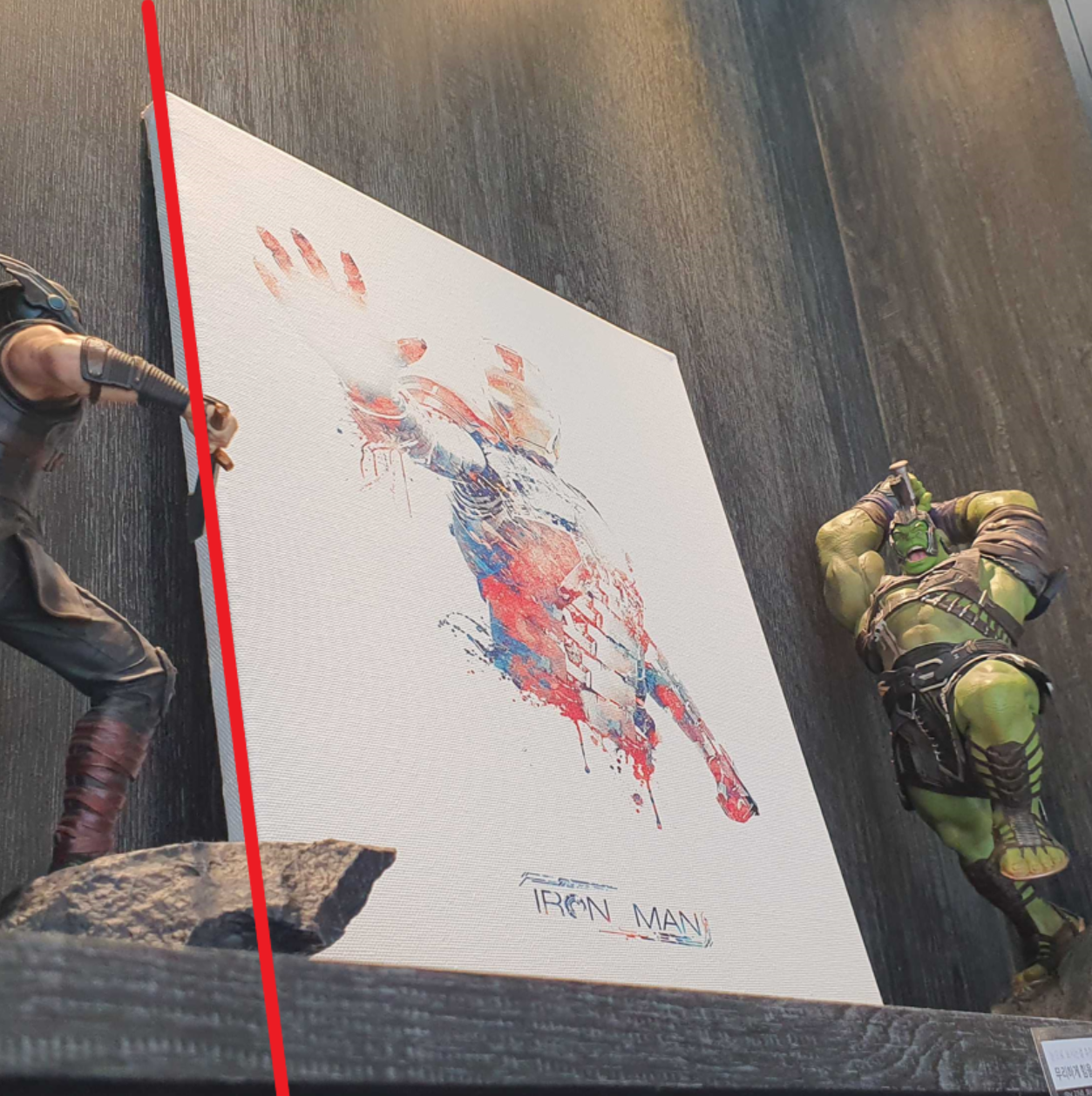
우선, 임의의 직사각형 물체를 촬영한 후 복원하고자하는 직선의 선분들의 픽셀 위치를 알아야 한다. 이 때, 직선들을 1,2,3,4 순서대로 코드에 잘 입력하는 것이 중요한데 헷갈리지 않기 위해 그림판 도구로 각 선분에 직선을 미리 그려본 후 각 직선의 픽셀 위치를 알아낸다. 예제 사진에서는 카메라의 렌즈로 인한 왜곡(lens distortion)은 무시한다.

Affine Rectification

affine 성질을 복원한다는 의미는 실제 세계에서 평행하지만 이미지 평면상에서 projective 변환에 의해 평행하지 않은 두 직선을 다시 복원한다는 의미이다.
임의의 affine homography $\mathbf{H}_{A}$가 affine 성질을 보존한다는 의미는 곧 무한대 직선 $\mathbf{l}_{\infty}$를 $\mathbf{H}_{A}$ 변환해도 무한대에 위치한 직선이 된다는 의미이다. 즉, 무한대 직선 위의 한 점 $\mathbf{x}_{\infty}$ 점이 있다고 했을 때 다음이 성립한다.
\begin{equation}
\begin{aligned}
\mathbf{H}_{A}(\mathbf{x}_{\infty}) = \mathbf{H}_{A}\mathbf{x}_{\infty} = \mathbf{x}_{\infty}^{\prime}
\end{aligned}
\end{equation}
무한대 직선 위의 한 점 $\mathbf{x}_{\infty}$는 $\mathbf{x}_{\infty}=(x,y,0)^{\intercal}$와 같이 마지막 항이 0인 특징이 있으므로 임의의 affine homography $\mathbf{H}_{A}$는
\begin{equation}
\begin{aligned}
\mathbf{H}_{A}\mathbf{x}_{\infty} = \begin{bmatrix} \mathbf{A}& \mathbf{t} \\ \mathbf {v} & v \end{bmatrix} \begin{bmatrix} x\\y\\0 \end{bmatrix} = \begin{bmatrix} *\\ * \\0 \end{bmatrix}
\end{aligned}
\end{equation}
이 성립하므로 $\mathbf{v}=(0,0)$이 되고 $v$는 스케일 상수가 되어 1로 변환이 가능하다.
\begin{equation}
\begin{aligned}
\mathbf{H}_{A} = \begin{bmatrix} \mathbf{A}&\mathbf{t} \\ \mathbf{0} & v \end{bmatrix} = \begin{bmatrix} \mathbf{A}/v & \mathbf{t}/v \\ \mathbf{0} & 1 \end{bmatrix}
\end{aligned}
\end{equation}
하지만 현실의 카메라를 통해 촬영한 영상에서는 projective 변환이 적용되므로 $\mathbf{l}_{\infty}$의 성질이 보존되지 않고 이미지 상에 투영된다.

따라서 위와 같이 투영된 임의의 직선 $\mathbf{l}^{'}$ (image of line at infinity)를 $\mathbf{l}_{\infty}$로 변환하는 homography $\mathbf{H}_{ar}$를 찾는 과정이 affine rectification이 된다.
$$\mathbf{H}_{ar}(\mathbf{l}^{'}) = \mathbf{H}_{ar}^{-\intercal}\mathbf{l}^{'} = \mathbf{l}_{\infty}$$

임의의 한 직선은 $\mathbf{l}^{'}=\begin{bmatrix} a & b & c \end{bmatrix}^{\intercal}$와 같이 나타낼 수 있고 $\mathbf{l}_{\infty}=\begin{bmatrix} 0 & 0 & 1 \end{bmatrix}^{\intercal}$ 이므로 이를 다시 표현하면 다음과 같다.
$$\mathbf{H}_{ar}(\mathbf{l}^{'}) = \mathbf{H}_{ar}^{-\intercal}\begin{bmatrix} a \\ b \\ c \end{bmatrix}=\begin{bmatrix} 0 \\ 0 \\ 1 \end{bmatrix}$$
다음으로 $\mathbf{H}_{ar}$의 성분을 찾아야 한다. 임의의 projective 변환 $\mathbf{H}_{p}$은 다음과 같이 3개의 서로 다른 homography로 분리할 수 있고
\begin{equation}
\begin{aligned}
\mathbf{H}_{p} & = \mathbf{H}_{S}\mathbf{H}_{A}\mathbf{H}_{P} \\
& = \begin{bmatrix} s \mathbf{R}&\mathbf{t} \\\mathbf{0}&1 \end{bmatrix} \begin{bmatrix} \mathbf{K} & \mathbf{0} \\ \mathbf{0} & 1 \end{bmatrix} \begin{bmatrix} \mathbf{I} & \mathbf{0}\\ \mathbf{v}^{\intercal}& v\end{bmatrix} \\
& = \begin{bmatrix} \mathbf{A}&\mathbf{t} \\ \mathbf{v}^{\intercal}&v \end{bmatrix}
\end{aligned}
\end{equation}
이 중, $\mathbf{H}_{P}$ 변환이 $\mathbf{l}_{\infty}$ 성질을 보존하지 않는 projective 변환의 성질을 지닌다. 따라서 $\mathbf{H}_{ar}$의 형태는 다음과 같다.
$$\mathbf{H}_{ar} = \begin{bmatrix} \mathbf{I} & \mathbf{0}\\ \mathbf{v}^{\intercal}& v\end{bmatrix}$$
위 형태를 만족하면서 $\mathbf{l}^{'}$를 $\mathbf{l}_{\infty}$로 변환시키는 $\mathbf{H}_{ar}$는 다음과 같다.
$$\mathbf{H}_{ar} = \begin{bmatrix} 1 & 0 & 0 \\ 0 & 1 & 0 \\ a & b & c\end{bmatrix}$$
$$\mathbf{H}_{ar}^{-\intercal}\mathbf{l}^{'} = \mathbf{l}_{\infty} = \begin{bmatrix} 1 & 0 & 0 \\ 0 & 1 & 0 \\ a & b & c\end{bmatrix}^{-\intercal}\begin{bmatrix} a \\ b \\ c \end{bmatrix}=\begin{bmatrix} 0 \\ 0 \\ 1 \end{bmatrix}$$
지금까지 affine rectification 순서를 정리하면 다음과 같다.
1. 실제 세계에서 평행한 직선 2쌍의 좌표를 구한다.
2. 평행한 직선 1쌍 당 소실점(=image of point at infinity) $\mathbf{v}$를 구한다. 총 2쌍이므로 2개 $\mathbf{v}_{1}, \mathbf{v}_{2}$를 구한다.
3. $\mathbf{v}_{1}$, $\mathbf{v}_{2}$를 잇는 image of line at infinity $\mathbf{l}^{'} = [a,b,c]^{\intercal}$를 구한다.
4. $\mathbf{l}^{'}$를 바탕으로 recover homography $\mathbf{H}_{ar}$를 구한다.
$$\mathbf{H}_{ar} = \begin{bmatrix} 1 & 0 & 0 \\ 0 & 1 & 0 \\ a & b & c\end{bmatrix}$$
5. 이미지 전체에 $\mathbf{H}_{ar}$를 적용하여 affine rectification을 마무리한다. affine rectification 결과 이미지는 평행한 선들이 보존된다.
Metric Rectification
metric성질을 복원한다는 의미는 실제 세계에서 수직이지만 이미지 평면상에서 projective 변환에 의해 직교하지 않은 두 직선을 다시 복원한다는 의미이다. 이 때, 복원된 이미지는 정확한 스케일 값까지는 알 수 없다(up to similarity, up to scale). 즉, metric rectification은 원본 이미지와 스케일 값만 다른 영상까지 복원한다는 의미이다. 이를 수행하기 위해서는 absolute dual conic $\mathbf{C}_{\infty}^{\ast}$의 특징을 사용하여 복원해야 한다.
Circular Point
circular point (또는 absolute point) $\mathbf{x}_{c}, \mathbf{x}_{-c}$는 다음과 같이 정의된다.
$$\mathbf{x}_{\pm c} = \begin{bmatrix} 1 \\ \pm i \\ 0 \end{bmatrix} \in \mathbb{CP}^{2}$$
- $i = \sqrt{-1}$
- $\mathbb{CP}^{2}$ : complex projective space
임의의 homography $\mathbf{H}$가 circular point 집합을 보존하면 $\mathbf{H}$는 simliarity 성질을 보존하는 특징이 있다.
$$\mathbf{H}(\mathbf{x}_{\pm c}) = \mathbf{x}_{\pm c} \quad \text{then, } \mathbf{H} \in \mathbf{H}_{s}$$
따라서 $\mathbf{H}$의 형태는 다음과 같다.
$$\mathbf{H} = \begin{bmatrix} A & t \\ 0 & 1 \end{bmatrix} = \begin{bmatrix} s\mathbf{R} & t \\ 0 & 1 \end{bmatrix}$$
- $s$ : scale factor
- $\mathbf{R}$ : rotation matrix
Dual Conic Properties
$\mathbb{P}^{2}$ 공간 상의 두 점 $\mathbf{P}$, $\mathbf{Q}$가 존재할 때 두 점을 잇는 직선에 접하는 dual conic $\mathbf{C}^{\ast}$는 다음과 같이 나타낼 수 있다.
$$\mathbf{C}^{\ast} = \mathbf{P}\mathbf{Q}^{\intercal} + \mathbf{Q}\mathbf{P}^{\intercal}$$
- $\mathbf{P} = [p_1, p_2, p_3]^{\intercal}$
이 때, $\mathbf{C}^{\ast}$는 두 점 $\mathbf{P}$와 $\mathbf{Q}$를 지나는 직선 $\mathbf{l}$을 매개화하는 dual conic을 의미한다. dual conic과 $\mathbf{C}^{\ast}$과 이에 접하는 직선 $\mathbf{l}$은 다음과 같은 관계를 가진다.
$$\mathbf{l}^{\intercal}\mathbf{C}^{\ast}\mathbf{l} = 0$$
$$\mathbf{l}^{\intercal}(\mathbf{P}\mathbf{Q}^{\intercal} + \mathbf{Q}\mathbf{P}^{\intercal})\mathbf{l} = 0$$
직선 $\mathbf{l}$ 상에 두 점 $\mathbf{P}$와 $\mathbf{Q}$가 포함되므로 $\mathbf{P}^{\intercal}\mathbf{l}=0$ 또는 $\mathbf{Q}^{\intercal}\mathbf{l}=0$ 이 성립하여 위 식이 만족된다.
Absolute Dual Conic
absolute dual conic $\mathbf{C}^{\ast}_{\infty}$은 두 개의 circular point를 지나는 직선을 매개화하는 dual conic을 의미한다.
$$\mathbf{C}^{\ast}_{\infty} = \mathbf{x}_{c}\mathbf{x}_{-c}^{\intercal} + \mathbf{x}_{-c}\mathbf{x}_{c}^{\intercal}$$
$$\mathbf{C}^{\ast}_{\infty} = \begin{bmatrix} 1 \\ i \\ 0 \end{bmatrix}\begin{bmatrix} 1 & -i & 0 \end{bmatrix} + \begin{bmatrix} 1 \\ -i \\ 0 \end{bmatrix}\begin{bmatrix} 1 & i & 0 \end{bmatrix}$$
$$= \begin{bmatrix} 1 & 0 & 0 \\ 0 & 1 & 0 \\ 0 & 0 & 0 \end{bmatrix}$$
$\mathbb{P}^{2}$ 공간 상의 임의의 두 직선 $\mathbf{l}, \mathbf{l}'$ 이 존재할 때 두 직선의 각도는 다음과 같이 나타낼 수 있다.
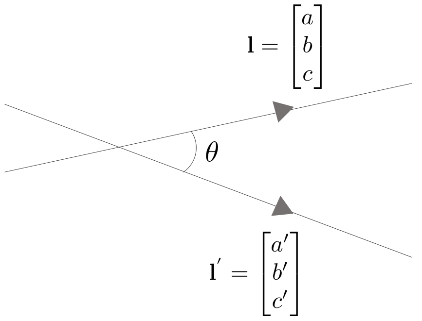
$$\cos\theta = \frac{aa' + bb'}{\sqrt{a^{2} + b^{2}}\sqrt{a'^{2} + b'^{2}}}$$
이 때, 위 식을 $\mathbf{C}^{\ast}_{\infty} = \begin{bmatrix} 1 & 0 & 0 \\ 0 & 1 & 0 \\ 0 & 0 & 0 \end{bmatrix}$를 사용하여 표현하면 다음과 같다.
$$\cos\theta = \frac{ \mathbf{l}^{\intercal}\mathbf{C}_{\infty}^{\ast}\mathbf{l}' }{ \sqrt{\mathbf{l}^{\intercal}\mathbf{C}_{\infty}^{\ast}\mathbf{l}} \sqrt{\mathbf{l}'^{\intercal}\mathbf{C}_{\infty}^{\ast}\mathbf{l}'} }$$
- $aa' + bb' = \mathbf{l}^{\intercal}\mathbf{C}_{\infty}^{\ast}\mathbf{l}'$
- $\sqrt{a^{2} + b^{2}} = \sqrt{\mathbf{l}^{\intercal}\mathbf{C}_{\infty}^{\ast}\mathbf{l}}$
- $\sqrt{a'^{2} + b'^{2}} = \sqrt{\mathbf{l}'^{\intercal}\mathbf{C}_{\infty}^{\ast}\mathbf{l}'}$
Homography of Dual Conic
dual conic과 $\mathbf{C}^{\ast}$과 이에 접하는 직선 $\mathbf{l}$은 다음과 같은 관계를 가진다.
$$\mathbf{l}^{\intercal}\mathbf{C}^{\ast}\mathbf{l} = 0$$
앞서 설명한 위 공식에 Homography $\mathbf{H}: \mathbb{P}^{2} \mapsto \mathbb{P}^{2}$를 수행하면 다음과 같다. $\mathbf{H}(\mathbf{l}) = \mathbf{H}^{-\intercal}\mathbf{l}$이므로
$$(\mathbf{H}^{-\intercal}\mathbf{l})^{\intercal} \mathbf{H}(\mathbf{C}^{\ast}) (\mathbf{H}^{-\intercal}\mathbf{l}) = 0$$
$$\therefore \mathbf{H}(\mathbf{C}^{\ast}) = \mathbf{H}\mathbf{C}^{\ast}\mathbf{H}^{\intercal}$$
이 때, $\mathbf{H}(\mathbf{C}^{\ast})$를 image of absolute dual conic $\mathbf{w}$라고 한다.
Image of Absolute Dual Conic
만약 $\mathbb{P}^{2}$ 공간 상에서 두 직선 $\mathbf{l}, \mathbf{m}$이 직교하면 다음과 같은 공식이 성립한다.
$$\mathbf{l}^{\intercal}\mathbf{w}\mathbf{m} = 0$$
- $\mathbf{w}$ : image of absolute conic $\mathbf{C}_{\infty}^{\ast}$
$\mathbf{w} = \mathbf{H}\mathbf{C}^{\ast}\mathbf{H}^{\intercal}$이므로 $\mathbf{H}$의 형태를 알기 위해 임의의 projective homography $\mathbf{H}$를 분해해보면 다음과 같다.
\begin{equation}
\begin{aligned}
\mathbf{H} & = \mathbf{H}_{S}\mathbf{H}_{A}\mathbf{H}_{P} \\
& = \begin{bmatrix} s \mathbf{R}&\mathbf{t} \\\mathbf{0}&1 \end{bmatrix} \begin{bmatrix} \mathbf{K} & \mathbf{0} \\ \mathbf{0} & 1 \end{bmatrix} \begin{bmatrix} \mathbf{I} & \mathbf{0}\\ \mathbf{v}^{\intercal}& v\end{bmatrix} \\
\end{aligned}
\end{equation}
$\mathbf{H}^{-1} = \mathbf{H}_{P}^{-1}\mathbf{H}_{A}^{-1}\mathbf{H}_{S}^{-1} = \mathbf{H}_{P}'\mathbf{H}_{A}'\mathbf{H}_{S}'$ 또한 동일한 homography 연산을 의미한다. 편의상 $\mathbf{H}_{P}'\mathbf{H}_{A}'\mathbf{H}_{S}'$을 $\mathbf{H}_{P}\mathbf{H}_{A}\mathbf{H}_{S}$라고 표기한다. 이 때, 각 행렬의 디테일한 $\mathbf{R},\mathbf{t},\mathbf{K},\mathbf{v}, s, v$ 값은 $\mathbf{H}$와 $\mathbf{H}^{-1}$이 서로 다르다. 따라서 $\mathbf{H}$의 decompose 순서를 반대로하여 곱해주어 $\mathbf{w}$를 전개해보면 다음과 같다.
$$\mathbf{H}\mathbf{C}^{\ast}\mathbf{H}^{\intercal} = \mathbf{H}_{P}\mathbf{H}_{A}\mathbf{H}_{S} \begin{bmatrix} 1&0&0 \\ 0&1&0 \\ 0&0&0 \end{bmatrix} \mathbf{H}_{S}^{\intercal}\mathbf{H}_{A}^{\intercal}\mathbf{H}_{P}^{\intercal}$$
$$\mathbf{H}\mathbf{C}^{\ast}\mathbf{H}^{\intercal} = \mathbf{H}_{P}\mathbf{H}_{A} \begin{bmatrix} 1&0&0 \\ 0&1&0 \\ 0&0&0 \end{bmatrix} \mathbf{H}_{A}^{\intercal}\mathbf{H}_{P}^{\intercal}$$
- $\because \mathbf{H}_{S} \begin{bmatrix} 1&0&0 \\ 0&1&0 \\ 0&0&0 \end{bmatrix} \mathbf{H}_{S}^{\intercal} = \begin{bmatrix} 1&0&0 \\ 0&1&0 \\ 0&0&0 \end{bmatrix}$
이를 전개하면 다음과 같다.
$$\mathbf{w} = \begin{bmatrix} \mathbf{KK}^{\intercal} & \mathbf{KK}^{\intercal}\mathbf{v} \\ \mathbf{v}^{\intercal}\mathbf{K}^{\intercal}\mathbf{K} & \mathbf{v}^{\intercal}\mathbf{KK}^{\intercal}\mathbf{v} \end{bmatrix}$$
최종적으로 projective 변환이 없는 similarity 변환이라고 가정하면 $\mathbf{v} = 0$이 되고 $\mathbf{w}$는 다음과 같다.
$$\mathbf{w} = \begin{bmatrix} \mathbf{KK}^{\intercal} & 0 \\ 0 & 0 \end{bmatrix}$$
Metric Rectification
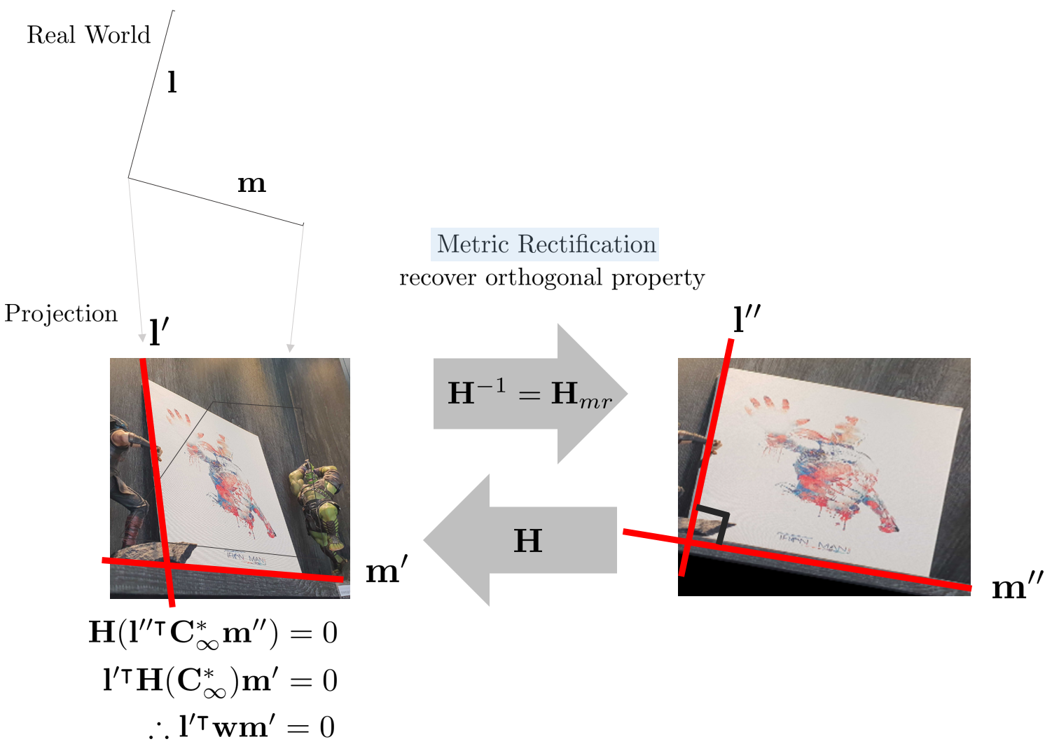
앞서 언급한 내용과 같이 $\mathbf{H}$에 의한 image of absolute dual conic은 $\mathbf{w} = \begin{bmatrix} \mathbf{KK}^{\intercal} & 0 \\ 0 & 0 \end{bmatrix}$로 나타낼 수 있다. 따라서 위 그림에서 $\mathbf{l}''$, $\mathbf{m}''$에 homography 변환 $\mathbf{H}$를 적용한 결과는 다음과 같이 나타낼 수 있다.
$$\mathbf{H}(\mathbf{l}''\mathbf{C}^{\ast}_{\infty}\mathbf{m}'') = \mathbf{l}'\mathbf{w}\mathbf{m}' = 0$$
- $\mathbf{H}(\mathbf{l}'') = \mathbf{l}'$
- $\mathbf{H}(\mathbf{C}_{\infty}^{\ast}) = \mathbf{w}$
- $\mathbf{H}(\mathbf{m}'') = \mathbf{m}'$
이를 다시 전개하면
$$\mathbf{l}'\begin{bmatrix} \mathbf{KK}^{\intercal} & 0 \\ 0 & 0 \end{bmatrix}\mathbf{m}' = 0$$
$$\begin{bmatrix} l'_{1} & l'_{2} \end{bmatrix} \mathbf{KK}^{\intercal} \begin{bmatrix} m'_{1} \\ m'_{2} \end{bmatrix} = 0$$
- $\mathbf{KK}^{\intercal} \in \mathbb{R}^{2\times2}$ : symmetric matrix & $\det \mathbf{KK}^{\intercal} = 1$
따라서 2개의 수직인 직선 쌍으로부터 $\mathbf{KK}^{\intercal}$을 계산하여 $\mathbf{w}$를 구할 수 있다. $\mathbf{KK}^{\intercal} = \mathbf{S}$로 치환했을 때, symmetric이고 positive definite 행렬은 다음과 같이 분해될 수 있다.
$$\begin{bmatrix} l'_{1} & l'_{2} \end{bmatrix} \mathbf{S} \begin{bmatrix} m'_{1} \\ m'_{2} \end{bmatrix} = 0$$
$$\mathbf{S} = \mathbf{UDU}^{\intercal}$$
- $\mathbf{U}$ : orthogonal matrix
- $\mathbf{D}$ : diagonal matrix
다시 diagonal matrix $\mathbf{D}$는 2개의 행렬의 곱 $\mathbf{D} = \mathbf{EE}^{\intercal}$로 나타낼 수 있으므로 이를 다시 정리하면
$$\mathbf{S} = \mathbf{UE}(\mathbf{UE})^{\intercal}$$
다음으로 $\mathbf{UE}$를 QR decomposition을 수행하면 upper triangle 행렬 $\mathbf{R}(=\mathbf{K})$와 orthogonal 행렬 $\mathbf{Q}$로 분해할 수 있다. 이를 다시 전개하면 다음과 같다.
$$\mathbf{S} = \mathbf{KQ}\mathbf{Q}^{\intercal}\mathbf{K}^{\intercal} = \mathbf{KK}^{\intercal}$$
- $\mathbf{QQ}^{\intercal} = \mathbf{I}$
다음으로 $\mathbf{S}$를 cholesky 또는 SVD를 통해 $\mathbf{K}$를 추출하여 최종적인 metric rectify homography $\mathbf{H}^{-1} = \mathbf{H}_{mr}$를 구한다.
$$\mathbf{H}= \begin{bmatrix} \mathbf{K} & 0 \\ 0 & 1 \end{bmatrix}$$
$$\mathbf{H}_{mr} = \mathbf{H}^{-1}= \begin{bmatrix} \mathbf{K} & 0 \\ 0 & 1 \end{bmatrix}^{-1}$$
지금까지 metric rectification 순서를 정리하면 다음과 같다.
1. 서로 수직인 직선 쌍 $\mathbf{l}', \mathbf{m}'$를 선정하여 두 직선의 좌표를 구한다.
2. $\begin{bmatrix} l'_{1} & l'_{2} \end{bmatrix} \mathbf{S} \begin{bmatrix} m'_{1} \\ m'_{2} \end{bmatrix} = 0$ 공식을 통해 $\mathbf{S} = \mathbf{KK}^{\intercal}$을 구한다.
3. cholesky 또는 SVD를 통해 $\mathbf{K}$를 구하고 이를 통해 $\mathbf{H}_{mr} = \begin{bmatrix} \mathbf{K} & 0 \\ 0 & 1 \end{bmatrix}^{-1}$를 구한다.
4. 이미지에 $\mathbf{H}_{mr}$를 적용하여 metric rectification을 수행한다. 복원된 이미지는 원본 이미지와 스케일 값을 제외하고 동일한 형태를 지닌다(up to scale)
Code Review
예제 코드는 링크를 클릭하여 다운로드하면 된다. 전체 코드는 다음과 같다.
#include "util.h"

#include <Eigen/Dense>

#include <opencv2/core/core.hpp>
#include <opencv2/core/eigen.hpp>
#include <opencv2/highgui/highgui.hpp>
#include <opencv2/opencv.hpp>

#include <iostream>
#include <string>
#include <vector>

void ApplyHomography(cv::Mat &img, cv::Mat &img_out, Eigen::Matrix3d H) {
  cv::Mat _H;
  cv::eigen2cv(H, _H);
  cv::warpPerspective(img, img_out, _H,
                      cv::Size(img.size().width * 4, img.size().height * 1));
}

int main() {
  std::string fn_img =
      util::GetProjectPath() + "/picture/affine_metric_rectification/01.png";
  cv::Mat img = cv::imread(fn_img, 1);

  Eigen::Matrix<double, 8, 3> line_points;

  line_points <<
	  113, 5, 1,
	  223, 846, 1,
	  435, 2, 1,
	  707, 843, 1,
	  2, 706, 1,
	  841, 780, 1,
	  4, 6, 1,
	  841, 445, 1;

  Eigen::Matrix<double, 4, 3> lines;
  for (int i = 0; i < 8; i += 2) {
    Eigen::Vector3d v1, v2;
    v1 = line_points.row(i);
    v2 = line_points.row(i + 1);

    lines.row(i / 2) = v1.cross(v2);
  }

  // Affine Rectification-------------------
  // intersection of line #1 and #2.
  Eigen::Matrix<double, 2, 3> A;
  A << lines.row(0), lines.row(1);
  Eigen::FullPivLU<Eigen::MatrixXd> lu(A);
  Eigen::Vector3d nullspace1 = lu.kernel();
  nullspace1 = nullspace1 / nullspace1(2);

  // intersection of line #3 and #4.
  Eigen::Matrix<double, 2, 3> A2;
  A2 << lines.row(2), lines.row(3);
  Eigen::FullPivLU<Eigen::MatrixXd> lu2(A2);
  Eigen::Vector3d nullspace2 = lu2.kernel();
  nullspace2 = nullspace2 / nullspace2(2);

  // image of line at infinity.
  Eigen::Matrix<double, 2, 3> A3;
  A3 << nullspace1.transpose(), nullspace2.transpose();
  Eigen::FullPivLU<Eigen::MatrixXd> lu3(A3);
  Eigen::Vector3d image_of_line_at_inf = lu3.kernel();

  Eigen::Matrix3d H_ar;
  H_ar << 1, 0, 0, 0, 1, 0, image_of_line_at_inf.transpose();

  // affine rectification.
  cv::Mat img_aff;
  ApplyHomography(img, img_aff, H_ar);
  cv::resize(img_aff, img_aff, cv::Size(), 0.25, 0.25);
  cv::imshow("affine", img_aff);
  cv::waitKey(1);

  // Metric Rectification-------------------
  lines.row(0) /= lines.row(0)(2);
  lines.row(1) /= lines.row(1)(2);
  lines.row(2) /= lines.row(2)(2);
  lines.row(3) /= lines.row(3)(2);

  // remove last colmun.
  Eigen::Vector3d l1 = lines.row(0);
  Eigen::Vector3d l2 = lines.row(1);
  Eigen::Vector3d m1 = lines.row(3);
  Eigen::Vector3d m2 = lines.row(2);

  Eigen::Matrix<double, 2, 3> ortho_constraint;
  ortho_constraint <<
	  l1(0) * m1(0),
	  l1(0) * m1(1) + l1(1) * m1(0),
      l1(1) * m1(1),

	  l2(0) * m2(0),
	  l2(0) * m2(1) + l2(1) * m2(0),
      l2(1) * m2(1);

  Eigen::JacobiSVD<Eigen::Matrix<double, 2, 3>> svd(
      ortho_constraint, Eigen::ComputeFullU | Eigen::ComputeFullV);
  Eigen::Vector3d s = svd.matrixV().col(svd.matrixV().cols() - 1);
  Eigen::Matrix2d S;
  S << s(0), s(1),
	s(1), s(2);

  Eigen::JacobiSVD<Eigen::Matrix2d> svd2(S, Eigen::ComputeFullU |
                                                Eigen::ComputeFullV);
  Eigen::MatrixXd U = svd2.matrixU();
  Eigen::MatrixXd D = svd2.singularValues().asDiagonal();
  Eigen::Matrix2d K = U * D.cwiseSqrt() * U.transpose();

  Eigen::Matrix3d H_mr;
  H_mr <<
	  K(0, 0), K(0, 1), 0,
	  K(1, 0), K(1, 1), 0,
	  0, 0, 1;

  // metric rectification.
  cv::Mat img_metric;
  ApplyHomography(img, img_metric, H_mr.inverse() * H_ar);
  cv::resize(img_metric, img_metric, cv::Size(), 0.25, 0.25);
  cv::imshow("metric", img_metric);
  cv::moveWindow("metric", 1000, 0);
  cv::waitKey(0);

  return 0;
}
How to run
본 예제코드는 cmake 프로젝트로 작성하였으며 Ubuntu 18.04, cmake 3.16, opencv 4.2, eigen 3.3.7 버전에서 정상 작동하는 것을 확인하였다. 다음 순서로 프로그램을 빌드 및 실행하면 된다.
# clone the repository
$ git clone https://github.com/gyubeomim/mvg-example
$ cd mvg-example/affine-metric-rect

# cmake build
$ mkdir build
$ cd build
$ cmake ..
$ make

# run example
$ ./affine_metric_rectification
Code #1
void ApplyHomography(cv::Mat &img, cv::Mat &img_out, Eigen::Matrix3d H) {
  cv::Mat _H;
  cv::eigen2cv(H, _H);
  cv::warpPerspective(img, img_out, _H,
                      cv::Size(img.size().width * 4, img.size().height * 1));
}
이미지 상의 모든 점을 homography 변환하는 함수이다. eigen 행렬로 구한 $\mathbf{H}$를 opencv 행렬로 바꾼 후 이미지를 homography 변환한다.
$$\sum_{i}\mathbf{H}(\mathbf{x}_{i})$$
- $i$ : all pixel points in image
Code #2
int main() {
  std::string fn_img =
      util::GetProjectPath() + "/picture/affine_metric_rectification/01.png";
  cv::Mat img = cv::imread(fn_img, 1);

  Eigen::Matrix<double, 8, 3> line_points;

  line_points <<
	  113, 5, 1,
	  223, 846, 1,
	  435, 2, 1,
	  707, 843, 1,
	  2, 706, 1,
	  841, 780, 1,
	  4, 6, 1,
	  841, 445, 1;

  Eigen::Matrix<double, 4, 3> lines;
  for (int i = 0; i < 8; i += 2) {
    Eigen::Vector3d v1, v2;
    v1 = line_points.row(i);
    v2 = line_points.row(i + 1);

    lines.row(i / 2) = v1.cross(v2);
  }
  ...
예제 이미지를 불러온 후 이미지 상의 4개의 직선을 구하기 위해 8개의 점의 좌표를 line_points 변수에 입력한다. 이 때, 점들은 $\mathbb{P}^{2}$ 공간 상의 점이므로 $\mathbf{x} = [a,b,1]$ 형태로 마지막의 1 값을 추가하여 입력한다. 따라서 총 8x3개의 데이터가 line_points 변수에 저장된다.
다음으로 lines 변수에 4개의 직선을 넣는다. 두 점 $v_{1}, v_{2}$의 cross product는 직선 $\mathbf{l}_{i}$을 의미하므로
$$v_{1} \times v_{2} = \mathbf{l}_{i}$$
를 사용하여 4개의 직선을 구한 후 lines 변수에 넣어준다.
Code #3
  int main() {
      ...
      // Affine Rectification-------------------
      // intersection of line #1 and #2.
      Eigen::Matrix<double, 2, 3> A;
      A << lines.row(0), lines.row(1);
      Eigen::FullPivLU<Eigen::MatrixXd> lu(A);
      Eigen::Vector3d nullspace1 = lu.kernel();
      nullspace1 = nullspace1 / nullspace1(2);

      // intersection of line #3 and #4.
      Eigen::Matrix<double, 2, 3> A2;
      A2 << lines.row(2), lines.row(3);
      Eigen::FullPivLU<Eigen::MatrixXd> lu2(A2);
      Eigen::Vector3d nullspace2 = lu2.kernel();
      nullspace2 = nullspace2 / nullspace2(2);

      // image of line at infinity.
      Eigen::Matrix<double, 2, 3> A3;
      A3 << nullspace1.transpose(), nullspace2.transpose();
      Eigen::FullPivLU<Eigen::MatrixXd> lu3(A3);
      Eigen::Vector3d image_of_line_at_inf = lu3.kernel();

      Eigen::Matrix3d H_ar;
      H_ar << 1, 0, 0, 0, 1, 0, image_of_line_at_inf.transpose();

      // affine rectification.
      cv::Mat img_aff;
      ApplyHomography(img, img_aff, H_ar);
      cv::resize(img_aff, img_aff, cv::Size(), 0.25, 0.25);
      cv::imshow("affine", img_aff);
      cv::waitKey(1);
	  ...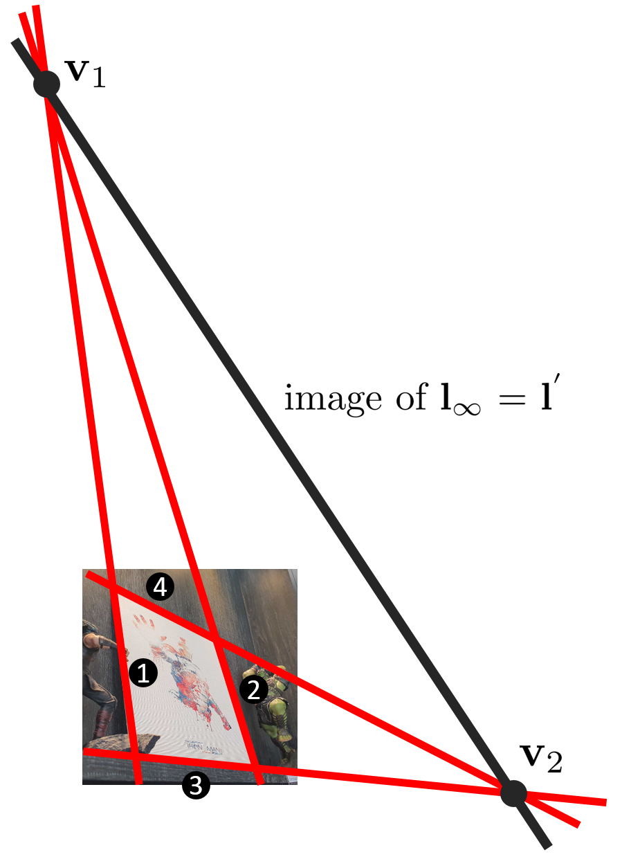
다음으로 소실점 $\mathbf{v}_{1}, \mathbf{v}_{2}$를 찾아야 한다. 1,2번 직선과 3,4번 직선은 각각 서로 평행하므로 두 직선의 교점이 line at infinity $\mathbf{l}_{\infty}$에서 만나야하지만 projective 변환된 이미지의 경우 두 직선들의 교점은 이미지 평면 상에서 만난다.
소실점 $\mathbf{v}_{1} = [v_{11}, v_{12}, v_{13}]^{\intercal}$을 구하기 위해 두 직선 $\mathbf{l}_{1} = [a_1, b_1, c_1]^{\intercal}, \mathbf{l}_{2} = [a_2, b_2, c_2]^{\intercal}$는 다음과 같이 나타낼 수 있다.
$$\begin{bmatrix} a_1 & b_1 & c_1 \\ a_2 & b_2 & c_2 \end{bmatrix} \begin{bmatrix} v_{11} \\ v_{12} \\ v_{13} \end{bmatrix} = \mathbf{0}$$
- $\mathbf{l}_{1}^{\intercal}\mathbf{v}_{1} = 0$ : a point on line
- $\mathbf{l}_{2}^{\intercal}\mathbf{v}_{1} = 0$ : a point on line
따라서 해당 선형시스템의 null space를 찾으면 이는 곧 $\mathbf{v}_{1}$의 해가 된다. $\mathbf{v}_{2}$도 $\mathbf{l}_{3}, \mathbf{l}_{4}$를 사용하여 똑같이 구한다. (nullspace1, nullspace2 변수)
다음으로 image of line at infinity $\mathbf{l}'$를 구해야 한다. 두 소실점 $\mathbf{v}_{1}, \mathbf{v}_{2}$를 잇는 직선이 곧 $\mathbf{l}' = [l'_1, l'_2, l'_3]^{\intercal}$를 의미하므로
$$\begin{bmatrix} v_{11} & v_{12} & v_{13} \\ v_{21} & v_{22} & v_{23} \end{bmatrix} \begin{bmatrix} l'_1 \\ l'_2 \\ l'_3 \end{bmatrix} = \mathbf{0}$$
- $\mathbf{v}_{1}^{\intercal}\mathbf{l}' = 0$ : a point on line
- $\mathbf{v}_{2}^{\intercal}\mathbf{l}' = 0$ : a point on line
따라서 해당 선형시스템의 null space를 찾으면 이는 곧 $\mathbf{l}'$의 해가 된다 (image_of_line_at_inf 변수). $\mathbf{l}' = [l'_1, l'_2, l'_3]^{\intercal}$를 구했으면 affine rectification homograhpy $\mathbf{H}_{ar}$를 다음과 같이 설정한다.
$$\mathbf{H}_{ar} = \begin{bmatrix} 1 & 0 & 0 \\ 0 & 1 & 0 \\ l'_1 & l'_2 & l'_3 \end{bmatrix}$$
최종적으로 원본 이미지에 $\mathbf{H}_{ar}$를 적용하면 affine rectification된 이미지를 얻을 수 있다.
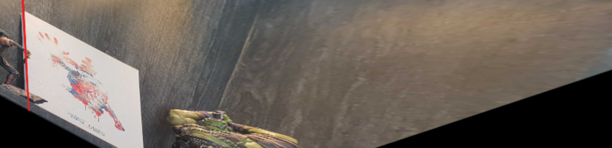
affine rectification을 수행하면 위 그림과 같이 평행한 선들이 보존되는 것을 확인할 수 있다.
Code #4
int main() {
	  ...
     // Metric Rectification-------------------
      lines.row(0) /= lines.row(0)(2);
      lines.row(1) /= lines.row(1)(2);
      lines.row(2) /= lines.row(2)(2);
      lines.row(3) /= lines.row(3)(2);

      // remove last colmun.
      Eigen::Vector3d l1 = lines.row(0);
      Eigen::Vector3d l2 = lines.row(1);
      Eigen::Vector3d m1 = lines.row(3);
      Eigen::Vector3d m2 = lines.row(2);

      Eigen::Matrix<double, 2, 3> ortho_constraint;
      ortho_constraint <<
          l1(0) * m1(0),
          l1(0) * m1(1) + l1(1) * m1(0),
          l1(1) * m1(1),

          l2(0) * m2(0),
          l2(0) * m2(1) + l2(1) * m2(0),
          l2(1) * m2(1);

      Eigen::JacobiSVD<Eigen::Matrix<double, 2, 3>> svd(
          ortho_constraint, Eigen::ComputeFullU | Eigen::ComputeFullV);
      Eigen::Vector3d s = svd.matrixV().col(svd.matrixV().cols() - 1);
      Eigen::Matrix2d S;
      S << s(0), s(1),
        s(1), s(2);

      Eigen::JacobiSVD<Eigen::Matrix2d> svd2(S, Eigen::ComputeFullU |
                                                    Eigen::ComputeFullV);
      Eigen::MatrixXd U = svd2.matrixU();
      Eigen::MatrixXd D = svd2.singularValues().asDiagonal();
      Eigen::Matrix2d K = U * D.cwiseSqrt() * U.transpose();

      Eigen::Matrix3d H_mr;
      H_mr <<
          K(0, 0), K(0, 1), 0,
          K(1, 0), K(1, 1), 0,
          0, 0, 1;

      // metric rectification.
      cv::Mat img_metric;
      ApplyHomography(img, img_metric, H_mr.inverse() * H_ar);
      cv::resize(img_metric, img_metric, cv::Size(), 0.25, 0.25);
      cv::imshow("metric", img_metric);
      cv::moveWindow("metric", 1000, 0);
      cv::waitKey(0);

      return 0;
    }
다음으로 metric rectification을 수행하기 위해 앞서 구한 서로 직교하는 직선 두 쌍 $\mathbf{l}_{1} \perp \mathbf{l}_{2}$과 $\mathbf{l}_{3} \perp \mathbf{l}_{4}$를 사용한다. 이 때, 직선의 마지막 z축 값은 사용하지 않으므로 이를 정규화해주고 더이상 사용하지 않는다. $\mathbf{l}_{1} = [l_{11}, l_{12}, l_{13}]^{\intercal}$을 예로들면 다음과 같다.
$$\mathbf{l}_{1} = [l_{11}, l_{12}, l_{13}]^{\intercal} \mapsto [\frac{l_{11}}{l_{13}}, \frac{l_{12}}{l_{13}}]^{\intercal}$$
편의상 $\frac{l_{11}}{l_{13}}, \frac{l_{12}}{l_{13}}$은 각각 $l_{11}$, $l_{12}$로 치환한다. 다른 직선 $\mathbf{l}_{2},\mathbf{l}_{3},\mathbf{l}_{4}$에 대해서도 동일한 과정을 수행한다.
다음으로 $\begin{bmatrix} l_{11} & l_{12} \end{bmatrix} \mathbf{S} \begin{bmatrix} l_{21} \\ l_{22} \end{bmatrix} = 0$ 공식을 통해 $\mathbf{S} = \mathbf{KK}^{\intercal}$을 구해야 한다. 이 때, $\mathbf{K}$은 $2 \times 2$ 행렬이고 $\det{\mathbf{K}}=1$을 만족하는 upper-triangle 행렬이므로
$$\mathbf{K} = \begin{bmatrix} a & b \\ 0 & c \end{bmatrix}$$
와 같이 나타낼 수 있고 따라서 $\mathbf{KK}^{\intercal} = \begin{bmatrix} a^2+b^2 & bc \\ bc & c^2 \end{bmatrix}$이 된다. 서로 직교하는 직선 두 쌍에 대해 식을 전개해보면 다음 공식을 유도할 수 있다.
$$\begin{bmatrix} l_{11} & l_{12} \\ l_{31} & l_{32} \end{bmatrix} \mathbf{KK}^{\intercal} \begin{bmatrix} l_{21} & l_{22} \\ l_{41} & l_{42} \end{bmatrix} = 0$$
$$\Rightarrow \begin{matrix} s_1(l_{11}l_{21}) + s_2(l_{11}l_{22} + l_{12}l_{21}) + s_3(l_{12}l_{22}) = 0 \\ s_1(l_{31}l_{41}) + s_2(l_{31}l_{42} + l_{32}l_{41}) + s_3(l_{32}l_{42}) = 0 \end{matrix}$$
$$ \Rightarrow \begin{bmatrix} l_{11}l_{21} & (l_{11}l_{22} + l_{12}l_{21}) & l_{12}l_{22} \\ l_{31}l_{41} & (l_{31}l_{42} + l_{32}l_{41}) & l_{32}l_{42} \end{bmatrix} \begin{bmatrix} s_1 \\ s_2 \\ s_3 \end{bmatrix} = 0$$
- $\mathbf{S} = \begin{bmatrix} s_1 & s_2 \\ s_2 & s_3 \end{bmatrix} = \mathbf{KK}^{\intercal}$ : symmetric & positive definite matrix
이 때 전개되는 복잡한 수식들은 $s_1, s_2, s_3$로 단순화하였다(ortho_constraint 변수). 다음으로 위 선형시스템의 null space를 구하면 $\mathbf{S} = \mathbf{KK}^{\intercal}$의 해를 구할 수 있다. $\mathbf{KK}^{\intercal}$를 구했으면 cholesky 또는 SVD 등 다양한 행렬 분해 방법을 사용하여 $\mathbf{K}$를 구할 수 있다. 이 때, 예제 코드에서는 링크의 방법을 참고하여 SVD의 대칭행렬 & positive definite의 버전인 spectral decomposition 방법을 사용하였다. 따라서 $\mathbf{KK}^{\intercal} = \mathbf{U}\mathbf{D}^{2}\mathbf{U}^{\intercal}$이므로 $\mathbf{K} = \mathbf{UDU}^{\intercal}$을 통해 구할 수 있다. 이 때 계산되는 $\mathbf{K}$값은 decomposition 방법에 따라서 실제 $\mathbf{K}$ 값과 다르게 분해된다.
이를 통해 homography $\mathbf{H}$를 표현하면 다음과 같다.
$$\mathbf{H} = \begin{bmatrix} \mathbf{K} & 0 \\ 0 & 1 \end{bmatrix} = \begin{bmatrix} k_1 & k_2 & 0 \\ k_2 & k_3 & 0 \\ 0 & 0 & 1 \end{bmatrix}$$
따라서 최종적인 metric rectification homography $\mathbf{H}_{mr}$은 다음과 같이 구할 수 있다.
$$\mathbf{H}_{mr} = \mathbf{H}^{-1} = \begin{bmatrix} k_1 & k_2 & 0 \\ k_2 & k_3 & 0 \\ 0 & 0 & 1 \end{bmatrix}^{-1}$$
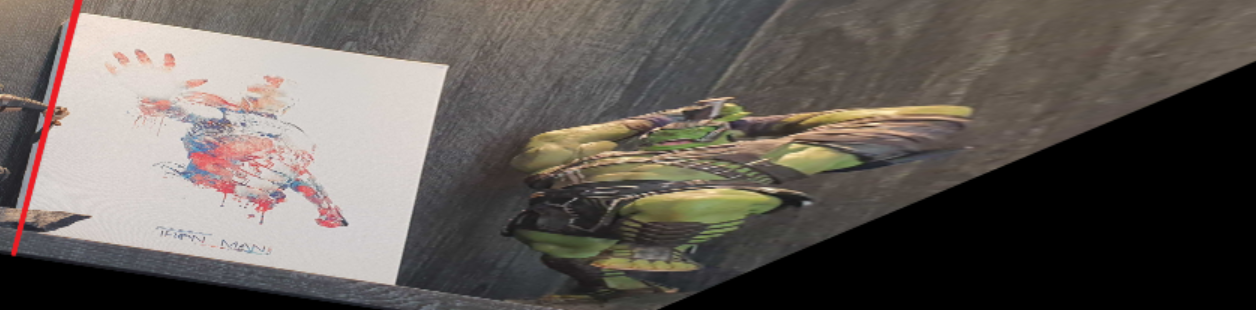
이를 affine rectification된 이미지에 적용하면 최종적으로 affine & metric rectification된 이미지를 얻을 수 있다. 이를 통해 실제 월드 상 물체와 동일하게 평행한 선과 직교한 선을 가지며 스케일 값을 제외하고(up to scale) 동일한 이미지를 얻을 수 있다.
'Engineering' 카테고리의 다른 글
| [MVG] Vanishing Point-based Metric Rectification 예제코드 및 설명 (C++) (0) | 2022.07.03 |
|---|---|
| [MVG] Zhang's Calibration 예제코드 및 설명 (C++) (0) | 2022.06.29 |
| [SLAM] g2o - Alternative Parameterizations 논문 섹션 리뷰 (0) | 2022.06.09 |
| [SLAM] g2o example 코드 리뷰 (0) | 2022.06.09 |
| [SLAM] Visual LiDAR Odometry and Mapping (V-LOAM) 논문 리뷰 (0) | 2022.06.08 |


