 A L I D A
해당 내용은 공부 목적으로 작성된 글입니다.
잘못된 부분이나 수정할 부분이 있다면 댓글이나 메일로 알려주시면 확인 후 수정하도록 하겠습니다.
본 포스트는 MVG part2 의 내용 중 "Image Rectification" 부분을 활용하여 두 이미지가 있을 때 이를 Stereo Camera Calibration(= Stereo Rectification) 수행하는 내용에 대해 리뷰한다. 또한 실제 스테레오 카메라를 캘리브레이션하는 방법에 대해서도 설명한다. 예제 코드는 우분투 18.04 환경에서 테스트하였으며 cmake 3.16, opencv 4.2, eigen 3.3.7 버전을 사용하여 정상적으로 작동하는 것을 확인하였다. 예제 코드는 링크를 클릭하여 다운로드하면 된다.
Stereo Camera Calibration
Why Stereo Rectification is necessary?

단일 이미지의 경우 특정 픽셀에 해당하는 맵포인트의 정확한 depth를 추정할 수 없는 반면, 2개의 이미지를 사용하게 되면 epipolar geometry를 사용하여 물체의 depth를 추정할 수 있다(e.g., triangulation). 하지만 왼쪽 이미지의 특정 포인트에 대응하는 대응점 쌍을 오른쪽 이미지에서 찾을 때 epipolar line을 계산해야 하는 추가 computational cost가 발생한다.
두 카메라가 동일한 orientation을 가지며 수평으로만 이동해있는 스테레오 이미지 상에서는 epipolar line이 서로 수평으로 정렬된다. epipolar line이 수평하게 정렬되면 왼쪽 이미지의 포인트에 해당하는 대응점 쌍을 오른쪽 이미지의 동일한 y축 픽셀 상에서 찾을 수 있기 때문에 computational cost가 감소하고 보다 비교적 단순하게 depth 추정이 가능한 이점이 있다. 스테레오 이미지에서 depth는 다음과 같이 구할 수 있다.
$$Z = \frac{bf}{D}$$

Input Image Setup
실제 월드 상에 존재하는 임의의 물체를 촬영한다. 이 때, 동일한 카메라를 사용하여 물체 기준 왼쪽에서 한 번, 오른쪽에서 한 번 씩 촬영한다. 촬영에 사용된 카메라는 갤럭시 노트10+를 사용하였다. 단순한 예제 구현을 위해 lens distortion은 없다고 가정하였다. 또한 두 이미지 상에서 대응점 쌍 8개를 이미 알고 있다고 가정한다. 그리고 zhang's method를 사용하여 카메라의 내부 파라미터 $\mathbf{K}$를 미리 알고 있다고 가정한다.

예제 코드와 달리 실제 stereo rectification을 수행할 때는 distortion parameter $k_1,k_2,p_1,p_2$를 구해서 렌즈에 의한 이미지 왜곡을 보정해줘야 한다. 이러한 실제 스테레오 카메라를 calibration하는 내용은 마지막 섹션에서 다룬다.
Stereo Rectification
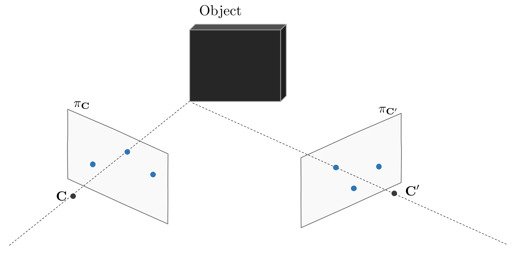
3차원 공간 상에 임의의 물체를 두 이미지 평면에서 촬영했다고 가정하자. 두 카메라의 기하학적 구조에 따라 생성되는 epipole과 epipolar line은 다음과 같다.

Stereo Rectification은 두 카메라의 이미지 평면 상의 epipolar line이 수평하도록 baseline을(=epipole을) 무한대로 보내는 과정을 의미한다. 자세한 과정은 다음과 같다.
1. 두 카메라의 대응점 쌍 8개를 사용하여 fundamental matrix $\mathbf{F}$를 구한다.
2. $\mathbf{E} = \mathbf{K}^{\intercal}\mathbf{F}\mathbf{K}$을 사용하여 essential matrix를 구한다. 이 때, intrinsic matrix $\mathbf{K}$는 미리 알고 있다고 가정한다.
3. $\mathbf{E} = \mathbf{t}^{\wedge}\mathbf{R}$의 특성을 사용하여 essential matrix를 분해하고 이를 통해 두 카메라 $\mathbf{C}, \mathbf{C}'$ 사이의 $\mathbf{R}, \mathbf{t}$를 구한다.
4. $\mathbf{R}^{-1}$을 $\mathbf{C}'$에 적용하여 $\mathbf{C}$와 동일한 방향을 보도록 회전시킨다.

5. baseline을 z 무한대 $[0, 0, 1]^{\intercal}$로 보내는 $\mathbf{R}_{rect}$를 구하여 이미지를 회전시키고 두 이미지 평면의 스케일을 조절하여 수평한 epipolar line들이 동일한 수평선 상에 있도록 조정한다.

실제 구현 상에서는 위 4,5번을 순차적으로 진행하지 않고 $\mathbf{H}_{1} = \mathbf{K}\mathbf{R}_{rect}\mathbf{K}^{-1}$, $\mathbf{H}_{2} = \mathbf{K}\mathbf{R}_{rect}\mathbf{R}^{\intercal}\mathbf{K}^{-1}$을 구하여 두 이미지 평면을 한번에 homography 변환한다.
$$\mathbf{x}_{i} = \mathbf{H}_{1}(\mathbf{x}_{i})$$
$$\mathbf{x}_{j} = \mathbf{H}_{2}(\mathbf{x}_{j})$$
- $i$ : left image's point
- $j$: right image's point
변환된 두 이미지는 다음 관계를 만족해야 한다.
$$\mathbf{R}_{lr} = \mathbf{I}, \quad \mathbf{t}_{lr} = [t_x, 0,0 ]^{\intercal}$$
- $\mathbf{R}_{lr}$ : rotation matrix from left to right camera
- $\mathbf{t}_{lr}$ : tranlsation vector from left to right camera
따라서 $\mathbf{E} = \mathbf{t}_{lr}^{\wedge}\mathbf{R}_{lr} = \begin{bmatrix} 0&0&0 \\ 0&0&-t_x \\ 0 & t_x & 0 \end{bmatrix}$을 만족하고 다음 공식 또한 만족한다.
$$\mathbf{x}^{\intercal} \mathbf{E} \mathbf{x}' = 0$$
이를 전개하면 다음과 같다.
$$\begin{bmatrix} u & v & 1 \end{bmatrix} \begin{bmatrix} 0&0&0 \\ 0&0&-t_x \\ 0 & t_x & 0 \end{bmatrix} \begin{bmatrix} u' \\ v' \\ 1 \end{bmatrix} = 0$$
$$\begin{bmatrix} u & v & 1 \end{bmatrix} \begin{bmatrix} 0 \\ -t_x \\ t_x v' \end{bmatrix} = 0$$
$$\therefore t_x v = t_x v'$$
즉, stereo rectified된 두 이미지는 대응점 쌍의 y축 좌표 ($v'$)가 항상 일치하는 것을 알 수 있다. 두 이미지 평면에서 8개의 대응점 쌍을 활용하여 fundamental matrix를 구한 후 이를 통해 epipolar line을 시각화하면 다음과 같다.

위 이미지에 stereo rectification을 적용하여 epipolar line을 수평하게 정렬한 결과는 아래와 같다. 해당 예제 이미지는 lens distortion을 고려하지 않고 stereo rectification을 수행해서 미세하게 두 이미지의 epipolar line들이 동일한 수평선 상에 있지 않지만 실제 stereo calibration을 수행할 때는 undistortion까지 수행하므로 epipolar line들이 동일한 수평선 상에 정렬된다.

Code Review
예제 코드는 링크를 클릭하여 다운로드하면 된다. 전체 코드는 다음과 같다.
#include "util.h"

#include <Eigen/Dense>

#include <opencv2/core/core.hpp>
#include <opencv2/core/eigen.hpp>
#include <opencv2/features2d.hpp>
#include <opencv2/highgui/highgui.hpp>
#include <opencv2/opencv.hpp>
#include <opencv2/features2d.hpp>

#include <iostream>
#include <numeric>
#include <random>
#include <string>
#include <vector>

using namespace std;

Eigen::Matrix3d CalculateFundamentalMatrix(Eigen::MatrixXd x1,
                                           Eigen::MatrixXd x2) {
  Eigen::Matrix3d F;

  // compute H1norm.
  double x1_mean_x = x1.col(0).mean();
  double x1_mean_y = x1.col(1).mean();
  Eigen::Vector2d centroid;
  centroid << x1_mean_x, x1_mean_y;

  std::vector<double> dist;
  for (int i = 0; i < x1.rows(); i++) {
    double d = std::sqrt((x1(i, 0) - centroid(0)) * (x1(i, 0) - centroid(0)) +
                         (x1(i, 1) - centroid(1)) * (x1(i, 1) - centroid(1)));
    dist.push_back(d);
  }

  double mean_dist = std::accumulate(dist.begin(), dist.end(), 0) / dist.size();

  Eigen::Matrix3d H1norm;
    H1norm << std::sqrt(2) / mean_dist, 0, -std::sqrt(2) / mean_dist * centroid(0),
	   	    0, std::sqrt(2) / mean_dist, -std::sqrt(2) / mean_dist * centroid(1),
	   		0, 0, 1;

  // compute H2norm.
  double x2_mean_x = x2.col(0).mean();
  double x2_mean_y = x2.col(1).mean();
  Eigen::Vector2d centroid2;
  centroid2 << x2_mean_x, x2_mean_y;

  std::vector<double> dist2;
  for (int i = 0; i < x2.rows(); i++) {
    double d = std::sqrt((x2(i, 0) - centroid2(0)) * (x2(i, 0) - centroid2(0)) +
                         (x2(i, 1) - centroid2(1)) * (x2(i, 1) - centroid2(1)));
    dist2.push_back(d);
  }

  double mean_dist2 =
      std::accumulate(dist2.begin(), dist2.end(), 0) / dist2.size();

  Eigen::Matrix3d H2norm;
    H2norm << std::sqrt(2) / mean_dist2, 0, -std::sqrt(2) / mean_dist2 * centroid2(0),
	  	    0, std::sqrt(2) / mean_dist2, -std::sqrt(2) / mean_dist2 * centroid2(1),
	  		0, 0, 1;

  x1 = (H1norm * x1.transpose()).transpose();
  x2 = (H2norm * x2.transpose()).transpose();

  // estimate fundamental matrix.
  Eigen::MatrixXd A(8, 9);
  A.col(0) = x1.col(0).cwiseProduct(x2.col(0));
  A.col(1) = x1.col(1).cwiseProduct(x2.col(0));
  A.col(2) = x2.col(0);
  A.col(3) = x1.col(0).cwiseProduct(x2.col(1));
  A.col(4) = x1.col(1).cwiseProduct(x2.col(1));
  A.col(5) = x2.col(1);
  A.col(6) = x1.col(0);
  A.col(7) = x1.col(1);
  A.col(8) = Eigen::VectorXd::Ones(8);

  // first SVD to get F0
  Eigen::JacobiSVD<Eigen::MatrixXd> svd(A, Eigen::ComputeFullU |
                                               Eigen::ComputeFullV);
  Eigen::MatrixXd V = svd.matrixV();
  Eigen::VectorXd f = V.col(V.cols() - 1);
  // Eigen::Matrix3d F0 = Eigen::Map<Eigen::Matrix3d>(f.data());
  Eigen::Matrix3d F0;
  F0 << f(0), f(1), f(2), f(3), f(4), f(5), f(6), f(7), f(8);

  // second SVD to get F_norm
  Eigen::JacobiSVD<Eigen::Matrix3d> svd2(F0, Eigen::ComputeFullU |
                                                 Eigen::ComputeFullV);
  Eigen::Matrix3d D = svd2.singularValues().asDiagonal();
  D(2, 2) = 0;
  Eigen::Matrix3d F_norm = svd2.matrixU() * D * svd2.matrixV().transpose();

  // get final fundamental matrix.
  F = H2norm.transpose() * F_norm * H1norm;

  return F;
}

void DrawEpipolarLines(cv::Mat img_left, cv::Mat img_right, Eigen::MatrixXd x1,
                       Eigen::MatrixXd x2, Eigen::Matrix3d F) {

  std::vector<cv::Scalar> colors;
  colors.push_back(cv::Scalar(255, 0, 0));
  colors.push_back(cv::Scalar(0, 255, 0));
  colors.push_back(cv::Scalar(0, 0, 255));
  colors.push_back(cv::Scalar(255, 255, 0));
  colors.push_back(cv::Scalar(255, 0, 255));
  colors.push_back(cv::Scalar(0, 255, 255));
  colors.push_back(cv::Scalar(125, 125, 0));
  colors.push_back(cv::Scalar(125, 0, 125));

  const int pt1 = -5000;
  const int pt2 = +5000;

  for (int i = 0; i < x1.rows(); i++) {
    Eigen::Vector3d x2_vec = x2.row(i);
    Eigen::Vector3d epipolar_line_left = F.transpose() * x2_vec;
    double a_l = epipolar_line_left(0);
    double b_l = epipolar_line_left(1);
    double c_l = epipolar_line_left(2);
    cv::Point2f pt_l1(pt1, (-a_l * pt1 - c_l) / b_l);
    cv::Point2f pt_l2(pt2, (-a_l * pt2 - c_l) / b_l);

    Eigen::Vector3d x1_vec = x1.row(i);
    Eigen::Vector3d epipolar_line_right = F * x1_vec;
    double a_r = epipolar_line_right(0);
    double b_r = epipolar_line_right(1);
    double c_r = epipolar_line_right(2);
    cv::Point2f pt_r1(pt1, (-a_r * pt1 - c_r) / b_r);
    cv::Point2f pt_r2(pt2, (-a_r * pt2 - c_r) / b_r);

#if 0
    std::cout << "Left" << std::endl;
    std::cout << a_l << ", " << b_l << ", " << c_l << std::endl;
    std::cout << pt_l1 << ", " << pt_l2 << std::endl;
    std::cout << "Right" << std::endl;
    std::cout << a_r << ", " << b_r << ", " << c_r << std::endl;
    std::cout << pt_r1 << ", " << pt_r2 << std::endl;
    std::cout << "-------------------------------------------------" << std::endl;
#endif
    cv::circle(img_left, cv::Point(x1_vec(0), x1_vec(1)), 20, colors[i],
               cv::FILLED, 8, 0);
    cv::circle(img_right, cv::Point(x2_vec(0), x2_vec(1)), 20, colors[i],
               cv::FILLED, 8, 0);
    cv::line(img_left, pt_l1, pt_l2, colors[i], 2);
    cv::line(img_right, pt_r1, pt_r2, colors[i], 2);
  }

  std::cout << "F\n" << F.matrix() << std::endl;

#if 1
  cv::resize(img_left, img_left, cv::Size(), 0.25, 0.25);
  cv::resize(img_right, img_right, cv::Size(), 0.25, 0.25);
  cv::imshow("epi_left", img_left);
  cv::imshow("epi_right", img_right);
  cv::moveWindow("epi_right", 1000, 0);
  cv::waitKey(1);
#endif
}


Eigen::MatrixXd Triangulation(Eigen::Matrix<double, 3, 4> P1,
                              Eigen::Matrix<double, 3, 4> P2,
                              Eigen::MatrixXd x1, Eigen::MatrixXd x2) {
  Eigen::MatrixXd X(1, 3);

  for (int i = 0; i < x1.rows(); i++) {
    Eigen::Matrix3d u_skew;
    u_skew << 0, -1, x1(i, 1), 1, 0, -x1(i, 0), -x1(i, 1), x1(i, 0), 0;
    Eigen::Matrix3d v_skew;
    v_skew << 0, -1, x2(i, 1), 1, 0, -x2(i, 0), -x2(i, 1), x2(i, 0), 0;

    Eigen::MatrixXd A(6, 4);
    A << u_skew * P1, v_skew * P2;

    Eigen::JacobiSVD<Eigen::MatrixXd> svd(A, Eigen::ComputeFullU |
                                                 Eigen::ComputeFullV);
    Eigen::MatrixXd V = svd.matrixV();
    X.row(i) = V.block<3, 1>(0, V.cols() - 1) / V(V.rows() - 1, V.cols() - 1);

    if (i != x1.rows() - 1) {
      X.conservativeResize(X.rows() + 1, X.cols());
    }
  }

  return X;
}

std::tuple<Eigen::Matrix3d, Eigen::Vector3d>
DecomposeFundamentalMatrix(Eigen::Matrix3d K, Eigen::Matrix3d F,
                           Eigen::MatrixXd x1, Eigen::MatrixXd x2) {
  Eigen::Matrix3d E = K.transpose() * F * K;

  Eigen::JacobiSVD<Eigen::Matrix3d> svd(E, Eigen::ComputeFullU |
                                               Eigen::ComputeFullV);

  Eigen::Matrix3d W;
  W << 0, -1, 0, 1, 0, 0, 0, 0, 1;
  Eigen::Vector3d t1 = svd.matrixU().col(2);
  Eigen::Matrix3d R1 = svd.matrixU() * W * svd.matrixV().transpose();
  if (R1.determinant() < 0) {
    t1 *= -1;
    R1 *= -1;
  }

  Eigen::Vector3d t2 = -svd.matrixU().col(2);
  Eigen::Matrix3d R2 = svd.matrixU() * W * svd.matrixV().transpose();
  if (R2.determinant() < 0) {
    t2 *= -1;
    R2 *= -1;
  }

  Eigen::Vector3d t3 = svd.matrixU().col(2);
  Eigen::Matrix3d R3 =
      svd.matrixU() * W.transpose() * svd.matrixV().transpose();
  if (R3.determinant() < 0) {
    t3 *= -1;
    R3 *= -1;
  }

  Eigen::Vector3d t4 = -svd.matrixU().col(2);
  Eigen::Matrix3d R4 =
      svd.matrixU() * W.transpose() * svd.matrixV().transpose();
  if (R4.determinant() < 0) {
    t4 *= -1;
    R4 *= -1;
  }

  // camera centers.
  Eigen::Vector3d T1 = -R1.transpose() * t1;
  Eigen::Vector3d T2 = -R2.transpose() * t2;
  Eigen::Vector3d T3 = -R3.transpose() * t3;
  Eigen::Vector3d T4 = -R4.transpose() * t4;

  // check four possible solutions.
  Eigen::Matrix<double, 3, 4> P1;
  P1 << K * Eigen::MatrixXd::Identity(3, 3),
      K * Eigen::VectorXd::Zero(3, 1);

  Eigen::Matrix<double, 3, 4> P2;
  P2 << K * R1 * Eigen::MatrixXd::Identity(3, 3), K * R1 * -T1;
  Eigen::MatrixXd X1 = Triangulation(P1, P2, x1, x2);

  P2 << K * R2 * Eigen::MatrixXd::Identity(3, 3), K * R2 * -T2;
  Eigen::MatrixXd X2 = Triangulation(P1, P2, x1, x2);

  P2 << K * R3 * Eigen::MatrixXd::Identity(3, 3), K * R3 * -T3;
  Eigen::MatrixXd X3 = Triangulation(P1, P2, x1, x2);

  P2 << K * R4 * Eigen::MatrixXd::Identity(3, 3), K * R4 * -T4;
  Eigen::MatrixXd X4 = Triangulation(P1, P2, x1, x2);

  std::vector<Eigen::Matrix3d> Rs;
  std::vector<Eigen::Vector3d> Ts;
  std::vector<Eigen::MatrixXd> Xs;

  Rs.push_back(R1);
  Rs.push_back(R2);
  Rs.push_back(R3);
  Rs.push_back(R4);

  Ts.push_back(T1);
  Ts.push_back(T2);
  Ts.push_back(T3);
  Ts.push_back(T4);

  Xs.push_back(X1);
  Xs.push_back(X2);
  Xs.push_back(X3);
  Xs.push_back(X4);

  // extract valid one solution.
  std::vector<int> valids(4);
  for (int i = 0; i < 4; i++) {
    int count = 0;

    for (int j = 0; j < Xs[i].rows(); j++) {
      Eigen::Vector3d Xs_vec = Xs[i].row(j);
      Eigen::VectorXd a = Rs[i].row(2) * (Xs_vec - Ts[i]);
      Eigen::VectorXd b = Xs[i].row(j).col(2);
      if (a.minCoeff() > 0 && b.minCoeff() > 0) {
        count += 1;
      }
    }
    valids[i] = count;
  }

  int best_idx =
      std::max_element(valids.begin(), valids.end()) - valids.begin();

  Eigen::Matrix3d R = Rs[best_idx];
  Eigen::Vector3d t = Ts[best_idx];

  return std::make_tuple(R, t);
}

std::tuple<Eigen::Matrix3d, Eigen::Matrix3d>
ComputeStereoHomography(Eigen::Matrix3d R, Eigen::Vector3d t,
                        Eigen::Matrix3d K) {
  Eigen::Vector3d rx, ry, rz, rz_tilde;

  rx = t / t.norm();
  rz_tilde << 0, 0, 1;

  Eigen::Vector3d tmp = rz_tilde - rz_tilde.dot(rx) * rx;
  rz = tmp / tmp.norm();
  ry = rz.cross(rx);

  Eigen::Matrix3d R_rect;
  R_rect << rx.transpose(), ry.transpose(), rz.transpose();

  Eigen::Matrix3d H1 = K * R_rect * K.inverse();
  Eigen::Matrix3d H2 = K * R_rect * R.transpose() * K.inverse();

  return std::make_tuple(H1, H2);
}

void ApplyHomography(cv::Mat &img, cv::Mat &img_out, Eigen::Matrix3d H) {
  cv::Mat _H;
  cv::eigen2cv(H, _H);
  cv::warpPerspective(img, img_out, _H, img.size());
}

int main() {
  std::string fn_left = util::GetProjectPath() + "/picture/left.jpg";
  std::string fn_right = util::GetProjectPath() + "/picture/right.jpg";

  cv::Mat img_left = cv::imread(fn_left, 1);
  cv::Mat img_right = cv::imread(fn_right, 1);

  Eigen::MatrixXd x1_best(8, 3);
  Eigen::MatrixXd x2_best(8, 3);

  x1_best <<
	    2201.606,  421.487, 1,
        2491.521, 1233.741, 1,
        2202.928, 294.5618, 1,
        1596.858, 621.5378, 1,
        2203.898,  1175.88, 1,
        2503.346,  1275.17, 1,
        2132.505, 298.8192, 1,
        2561.777, 745.0586, 1;

	x2_best <<
		 2404.31,  533.2378, 1,
         2403.97,  1370.911, 1,
        2450.759,  408.9355, 1,
        1749.202,  654.4105, 1,
        2140.022,  1267.529, 1,
        2399.647,   1413.43, 1,
         2380.94,  405.7941, 1,
        2653.428,  899.0267, 1;


  // load intrinsic parameter.
  Eigen::Matrix3d K;
  K << 2211.75963080077, 0, 2018.81623699895,
	   0,2218.36683671952, 1120.37532022008,
	   0, 0, 1;


  Eigen::Matrix3d F;
  F = CalculateFundamentalMatrix(x1_best, x2_best);

  DrawEpipolarLines(img_left, img_right, x1_best, x2_best, F);

  Eigen::Matrix3d R;
  Eigen::Vector3d t;

  std::tie(R, t) = DecomposeFundamentalMatrix(K, F, x1_best, x2_best);

  Eigen::Matrix3d H1;
  Eigen::Matrix3d H2;
  std::tie(H1, H2) = ComputeStereoHomography(R, t, K);

  cv::Mat img_left_warped, img_right_warped;
  ApplyHomography(img_left, img_left_warped, H1);
  ApplyHomography(img_right, img_right_warped, H2);

  cv::resize(img_left_warped, img_left_warped, cv::Size(), 0.25, 0.25);
  cv::resize(img_right_warped, img_right_warped, cv::Size(), 0.25, 0.25);
  cv::imshow("warped left", img_left_warped);
  cv::imshow("warped right", img_right_warped);
  cv::moveWindow("warped left", 0, 600);
  cv::moveWindow("warped right", 1000, 600);
  cv::waitKey(0);

  return 0;
}
DrawEpipolarLines() 함수는 이름 그대로 이미지에 epipolar line을 그려주는 함수이다. 해당 함수에 대한 자세한 설명은 생략한다.
How to run
본 예제코드는 cmake 프로젝트로 작성하였으며 Ubuntu 18.04, cmake 3.16, opencv 4.2, eigen 3.3.7 버전에서 정상 작동하는 것을 확인하였다. 다음 순서로 프로그램을 빌드 및 실행하면 된다.
# clone the repository
$ git clone https://github.com/gyubeomim/mvg-example
$ cd mvg-example/stereo-rectification

# cmake build
$ mkdir build
$ cd build
$ cmake ..
$ make

# run example
$ ./stereo
Code #1
Eigen::Matrix3d CalculateFundamentalMatrix(Eigen::MatrixXd x1,
                                           Eigen::MatrixXd x2) {
  Eigen::Matrix3d F;

  // compute H1norm.
  double x1_mean_x = x1.col(0).mean();
  double x1_mean_y = x1.col(1).mean();
  Eigen::Vector2d centroid;
  centroid << x1_mean_x, x1_mean_y;

  std::vector<double> dist;
  for (int i = 0; i < x1.rows(); i++) {
    double d = std::sqrt((x1(i, 0) - centroid(0)) * (x1(i, 0) - centroid(0)) +
                         (x1(i, 1) - centroid(1)) * (x1(i, 1) - centroid(1)));
    dist.push_back(d);
  }

  double mean_dist = std::accumulate(dist.begin(), dist.end(), 0) / dist.size();

  Eigen::Matrix3d H1norm;
    H1norm << std::sqrt(2) / mean_dist, 0, -std::sqrt(2) / mean_dist * centroid(0),
	   	    0, std::sqrt(2) / mean_dist, -std::sqrt(2) / mean_dist * centroid(1),
	   		0, 0, 1;

  // compute H2norm.
  double x2_mean_x = x2.col(0).mean();
  double x2_mean_y = x2.col(1).mean();
  Eigen::Vector2d centroid2;
  centroid2 << x2_mean_x, x2_mean_y;

  std::vector<double> dist2;
  for (int i = 0; i < x2.rows(); i++) {
    double d = std::sqrt((x2(i, 0) - centroid2(0)) * (x2(i, 0) - centroid2(0)) +
                         (x2(i, 1) - centroid2(1)) * (x2(i, 1) - centroid2(1)));
    dist2.push_back(d);
  }

  double mean_dist2 =
      std::accumulate(dist2.begin(), dist2.end(), 0) / dist2.size();

  Eigen::Matrix3d H2norm;
    H2norm << std::sqrt(2) / mean_dist2, 0, -std::sqrt(2) / mean_dist2 * centroid2(0),
	  	    0, std::sqrt(2) / mean_dist2, -std::sqrt(2) / mean_dist2 * centroid2(1),
	  		0, 0, 1;

  x1 = (H1norm * x1.transpose()).transpose();
  x2 = (H2norm * x2.transpose()).transpose();

  // estimate fundamental matrix.
  Eigen::MatrixXd A(8, 9);
  A.col(0) = x1.col(0).cwiseProduct(x2.col(0));
  A.col(1) = x1.col(1).cwiseProduct(x2.col(0));
  A.col(2) = x2.col(0);
  A.col(3) = x1.col(0).cwiseProduct(x2.col(1));
  A.col(4) = x1.col(1).cwiseProduct(x2.col(1));
  A.col(5) = x2.col(1);
  A.col(6) = x1.col(0);
  A.col(7) = x1.col(1);
  A.col(8) = Eigen::VectorXd::Ones(8);

  // first SVD to get F0
  Eigen::JacobiSVD<Eigen::MatrixXd> svd(A, Eigen::ComputeFullU |
                                               Eigen::ComputeFullV);
  Eigen::MatrixXd V = svd.matrixV();
  Eigen::VectorXd f = V.col(V.cols() - 1);
  // Eigen::Matrix3d F0 = Eigen::Map<Eigen::Matrix3d>(f.data());
  Eigen::Matrix3d F0;
  F0 << f(0), f(1), f(2), f(3), f(4), f(5), f(6), f(7), f(8);

  // second SVD to get F_norm
  Eigen::JacobiSVD<Eigen::Matrix3d> svd2(F0, Eigen::ComputeFullU |
                                                 Eigen::ComputeFullV);
  Eigen::Matrix3d D = svd2.singularValues().asDiagonal();
  D(2, 2) = 0;
  Eigen::Matrix3d F_norm = svd2.matrixU() * D * svd2.matrixV().transpose();

  // get final fundamental matrix.
  F = H2norm.transpose() * F_norm * H1norm;

  return F;
}
위 함수는 8개의 대응점 쌍을 이용하여 fundametal matrix $\mathbf{F}$를 구하는 함수이다. 두 카메라의 대응점쌍 $\mathbf{x} \leftrightarrow \mathbf{x}^{\prime}$이 존재할 때
\begin{equation}
\begin{aligned}
\mathbf{x}^{\prime\intercal}\mathbf{Fx} = 0
\end{aligned}
\end{equation}
을 만족하는 3x3 크기의 행렬 $\mathbf{F}$를 Fundamental Matrix라고 하며 $\mathbf{x}^{\prime\intercal}\mathbf{Fx}=0$이를 다시 정리하면 $\sum \mathbf{x}^{\prime}_{i}\mathbf{x}_{j}\mathbf{f}_{ij}=0$과 같이 정리할 수 있다. 해당 식은 선형시스템
\begin{equation}
\begin{aligned}
\mathbf{A} \mathbf{f} = 0
\end{aligned}
\end{equation}
꼴로 나타낼 수 있고 이 때 $\mathbf{A}$와 $\mathbf{f}$를 풀어쓰면 다음과 같다.
\begin{equation}
\begin{aligned}
& \mathbf{A} = (\mathbf{a}_{ik}) \in \mathbb{R}^{N \times 9}, \ \ \text{i-th row is} \ (\mathbf{x}_{1}^{\prime i}\mathbf{x}_{1}^{i}, \mathbf{x}_{1}^{\prime i}\mathbf{x}_{2}^{i},\cdots, \mathbf{x}_{n}^{\prime i}\mathbf{x}_{n}^{i}) \\
& \mathbf{f} = (\mathbf{f}_{11}, \mathbf{f}_{12}, \mathbf{f}_{13}, \cdots, \mathbf{f}_{33})^{\intercal} \in \mathbb{R}^{9\times 1} \\
& \mathbf{Af} = \begin{bmatrix} x'_{1}x_{1} & x'_{1}y_{1} & x'_{1} & y'_{1}x_{1} & y'_{1}y_{1} & y'_{1} & x_1 & y_1 & 1 \\ \vdots & \vdots & \vdots & \vdots & \vdots & \vdots & \vdots & \vdots \\ x'_{n}x_{n} & x'_{n}y_{n} & x'_{n} & y'_{n}x_{n} & y'_{n}y_{n} & y'_{n} & x_n & y_n & 1 \end{bmatrix} \mathbf{f} = 0
\end{aligned}
\end{equation}
- $\mathbf{x}_{k} = [x_{k}, y_{k}, 1]^{\intercal}$ : k-th left point
- $\mathbf{x}'_{k} = [x'_{k}, y'_{k}, 1]^{\intercal}$ : k-th right point
만약 주어진 대응점쌍의 개수 $n$이 8보다 크고 노이즈가 없는 완벽한 데이터로 생성이 되었으면 $\mathbf{A}$는 rank 8 행렬이 되고 유일한 해 $\mathbf{f}$가 존재한다. 이 때 $\mathbf{f}$는 $\mathbf{A}$의 Null Space의 원소가 된다. 하지만 대부분의 경우 주어진 데이터에는 항상 노이즈가 존재하므로 $\mathbf{A}$ 행렬은 rank 9인 full rank 행렬이 된다. 이 때 해를 구하면 $\mathbf{f}$는 항상 영벡터가 계산되므로 $\| \mathbf{f} \| = 1$이라는 조건하에 $\|\mathbf{Af}\|$의 크기를 최소화하는 근사해 $\mathbf{f}$를 찾아야 한다. 해를 찾는 방법은 $\mathbf{A}$를 특이값 분해(SVD)한 다음
\begin{equation}
\begin{aligned}
\mathbf{A} = \mathbf{UDV}^{\intercal}
\end{aligned}
\end{equation}
대각행렬 $\mathbf{D}$의 eigenvalue 중 가장 절대값이 작은 것에 대응되는 $\mathbf{V}$의 열벡터를 $\mathbf{f}$의 일반해로 간주한다. 해당 열벡터 $\mathbf{f}$가 $\|\mathbf{Af}\|$의 크기를 최소화하는 벡터가 되며 이를 Linear Solution이라고 부른다. 하지만 이 때, Linear Solution $\mathbf{f}$로 복원한 $\mathbf{F}_{0}$가 rank 2 행렬임을 보장할 수 없다. 수치적으로 해를 구하면 일반적으로 rank 3인 행렬이 나온다. 따라서 한 번 더 SVD를 사용하여 $\mathbf{F}_{0}$와 가장 가까운 rank 2 행렬을 찾아야 한다.
\begin{equation}
\begin{aligned}
\mathbf{F}_{0} = \mathbf{U}_{0}\mathbf{D}_{0}\mathbf{V}^{\intercal}_{0}
\end{aligned}
\end{equation}
이 때 대각행렬 $\mathbf{D}_{0} = \begin{bmatrix} \sigma_{1}&& \\ &\sigma_{2}& \\ &&\sigma_{3} \end{bmatrix}$는 일반적으로 마지막 특이값 $\sigma_{3}$가 0이 아니므로 rank 3인 행렬이 된다. 따라서 임의로 $\sigma_{3}=0$으로 변경한 행렬이 $\mathbf{F}_{0}$과 가장 가까운 rank 2 행렬이 된다.
The normalized 8-point algorithm
행렬 $\mathbf{A}$는 주어진 대응점쌍 $\mathbf{x} \leftrightarrow \mathbf{x}^{\prime}$으로 구성된 행렬이므로 대응점쌍들을 정규화(normalization)하지 않고 바로 해를 구하는 경우 $\mathbf{x}_{i} = (1000000,20000000,1)$과 같이 마지막 값에 비해서 처음 두 값의 크기가 매우 크게 되므로 수치적으로 불안정한 문제를 가진다. 따라서 $\mathbf{x}_{i}, \mathbf{x}_{i}^{\prime}$를 Centroid가 0이고 Centroid로부터 평균거리가 $\sqrt{2}$가 되도록하는 Homography 변환 $\mathbf{H}_{1}, \mathbf{H}_{2}$를 적용한다(H1norm, H2norm 변수).
\begin{equation}
\begin{aligned}
& \mathbf{x}_{i} \rightarrow \mathbf{H}_{1}\mathbf{x}_{i} \\
& \mathbf{x}_{i}^{\prime} \rightarrow \mathbf{H}_{2} \mathbf{x}_{i}^{\prime} \\
\end{aligned}
\end{equation}
이렇게 변환된 대응쌍점들을 사용하여 수치적으로 안정적인 Fundamental Matrix $\mathbf{F}^{\prime}$ 계산할 수 있다(F_norm 변수). 앞서 설명한 내용을 따라 $\mathbf{F}^{\prime}$를 계산한 다음 다시 원래의 대응점쌍 $\mathbf{x} \leftrightarrow \mathbf{x}^{\prime}$으로 복원하기 위해
\begin{equation}
\begin{aligned}
0 & = (\mathbf{H}_{2}\mathbf{x}^{\prime})^{\intercal}\mathbf{F}^{\prime}(\mathbf{H}_{1}\mathbf{x}) \\
& = \mathbf{x}^{\intercal}(\mathbf{H}_{2}^{\intercal} \mathbf{F}^{\prime}\mathbf{H}_{1})\mathbf{x}
\end{aligned}
\end{equation}
처럼 $\mathbf{F} = \mathbf{H}_{2}^{\intercal} \mathbf{F}^{\prime}\mathbf{H}_{1}$를 통해 원래 대응점쌍의 Fundamental Matrix $\mathbf{F}$를 계산할 수 있다.
Code #2
Eigen::MatrixXd Triangulation(Eigen::Matrix<double, 3, 4> P1,
                              Eigen::Matrix<double, 3, 4> P2,
                              Eigen::MatrixXd x1, Eigen::MatrixXd x2) {
  Eigen::MatrixXd X(1, 3);

  for (int i = 0; i < x1.rows(); i++) {
    Eigen::Matrix3d u_skew;
    u_skew << 0, -1, x1(i, 1), 1, 0, -x1(i, 0), -x1(i, 1), x1(i, 0), 0;
    Eigen::Matrix3d v_skew;
    v_skew << 0, -1, x2(i, 1), 1, 0, -x2(i, 0), -x2(i, 1), x2(i, 0), 0;

    Eigen::MatrixXd A(6, 4);
    A << u_skew * P1, v_skew * P2;

    Eigen::JacobiSVD<Eigen::MatrixXd> svd(A, Eigen::ComputeFullU |
                                                 Eigen::ComputeFullV);
    Eigen::MatrixXd V = svd.matrixV();
    X.row(i) = V.block<3, 1>(0, V.cols() - 1) / V(V.rows() - 1, V.cols() - 1);

    if (i != x1.rows() - 1) {
      X.conservativeResize(X.rows() + 1, X.cols());
    }
  }

  return X;
}
위 코드는 triangulation을 사용하여 3차원 월드 상의 점 $\mathbf{X} \in \mathbb{P}^{3}$를 구하는 함수이다. triangulation을 구하는 여러 방법 중 선형방정식을 사용하는 방법을 설명한다. $\mathbf{x}=\mathbf{PX}, \mathbf{x}^{\prime}=\mathbf{P}^{\prime}\mathbf{X}$로부터
\begin{equation}
\begin{aligned}
& \mathbf{x}^{\wedge}(\mathbf{PX}) = 0\\
& \mathbf{x}^{\prime\wedge}(\mathbf{P}^{\prime}\mathbf{X})=0
\end{aligned}
\end{equation}
공식이 성립한다.
\begin{equation}
\begin{aligned}
& \mathbf{x} = \begin{bmatrix} x&y&1 \end{bmatrix}^{\intercal} \\
& \mathbf{P} = \begin{bmatrix} \mathbf{p}_{1,row}^{\intercal} & \mathbf{p}_{2,row}^{\intercal} & \mathbf{p}_{3,row}^{\intercal} \end{bmatrix}^{\intercal} \\
& \mathbf{X} = \begin{bmatrix} X&Y&Z&W \end{bmatrix}^{\intercal}
\end{aligned}
\end{equation}
$\mathbf{p}_{i,row}^{\intercal}$를 $\mathbf{P}$의 i번째 행(row)라고 했을 때 $\mathbf{x}^{\wedge}(\mathbf{PX})$를 전개한 후 정리하면
\begin{equation}
\begin{aligned}
& x(\mathbf{p}_{3,row}^{\intercal}\mathbf{X}) - (\mathbf{p}_{1,row}^{\intercal}\mathbf{X}) = 0 \\
& y(\mathbf{p}_{3,row}^{\intercal}\mathbf{X}) - (\mathbf{p}_{2,row}^{\intercal}\mathbf{X}) = 0 \\
& x(\mathbf{p}_{2,row}^{\intercal}\mathbf{X}) - y(\mathbf{p}_{1,row}^{\intercal}\mathbf{X}) = 0 \\
\end{aligned}
\end{equation}
과 같고 이를 $\mathbf{x}^{\prime\wedge}(\mathbf{P}^{\prime}\mathbf{X})$도 같이 구한 후 $\mathbf{X}$에 대한 선형시스템으로 다시 작성하면
\begin{equation}
\begin{aligned}
& \underbrace{\begin{bmatrix}
x \mathbf{p}_{3,row}^{\intercal}-\mathbf{p}_{1,row}^{\intercal} \\
y \mathbf{p}_{3,row}^{\intercal}-\mathbf{p}_{2,row}^{\intercal} \\
x^{\prime} \mathbf{p}_{3,row}^{\prime\intercal}-\mathbf{p}_{1,row}^{\prime\intercal} \\
y^{\prime} \mathbf{p}_{3,row}^{\prime\intercal}-\mathbf{p}_{2,row}^{\prime\intercal} \\
\end{bmatrix}}_{\mathbf{A}}\mathbf{X} = 0 \\
\end{aligned}
\end{equation}
같이 $\mathbf{AX} = 0$ 형태로 정리할 수 있다. 데이터에 노이즈가 없는 경우 $\mathbf{A} \in \mathbb{R}^{4\times 4}$의 rank가 3이 되어 Null Space 벡터를 통해 유일한 $\mathbf{X}$를 계산할 수 있지만 노이즈가 존재하는 경우 $\mathbf{A}$의 rank는 4가 되어 무수히 많은 해가 존재한다. 따라서 $\mathbf{A}$를 특이값 분해(SVD)하여 $\|\mathbf{X} \|=1$일 때 $\|\mathbf{AX} \|$의 크기를 최소화하는 근사해 $\hat{\mathbf{X}}$를 계산해야 한다. X.row(i) = V.block<3, 1>(0, V.cols() - 1) / V(V.rows() - 1, V.cols() - 1) 부분이 $\|\mathbf{X} \|=1$로 만들기 위해 normalization을 수행하는 코드이다.
Code #3
std::tuple<Eigen::Matrix3d, Eigen::Vector3d>
DecomposeFundamentalMatrix(Eigen::Matrix3d K, Eigen::Matrix3d F,
                           Eigen::MatrixXd x1, Eigen::MatrixXd x2) {
  Eigen::Matrix3d E = K.transpose() * F * K;

  Eigen::JacobiSVD<Eigen::Matrix3d> svd(E, Eigen::ComputeFullU |
                                               Eigen::ComputeFullV);

  Eigen::Matrix3d W;
  W << 0, -1, 0, 1, 0, 0, 0, 0, 1;
  Eigen::Vector3d t1 = svd.matrixU().col(2);
  Eigen::Matrix3d R1 = svd.matrixU() * W * svd.matrixV().transpose();
  if (R1.determinant() < 0) {
    t1 *= -1;
    R1 *= -1;
  }

  Eigen::Vector3d t2 = -svd.matrixU().col(2);
  Eigen::Matrix3d R2 = svd.matrixU() * W * svd.matrixV().transpose();
  if (R2.determinant() < 0) {
    t2 *= -1;
    R2 *= -1;
  }

  Eigen::Vector3d t3 = svd.matrixU().col(2);
  Eigen::Matrix3d R3 =
      svd.matrixU() * W.transpose() * svd.matrixV().transpose();
  if (R3.determinant() < 0) {
    t3 *= -1;
    R3 *= -1;
  }

  Eigen::Vector3d t4 = -svd.matrixU().col(2);
  Eigen::Matrix3d R4 =
      svd.matrixU() * W.transpose() * svd.matrixV().transpose();
  if (R4.determinant() < 0) {
    t4 *= -1;
    R4 *= -1;
  }

  // camera centers.
  Eigen::Vector3d T1 = -R1.transpose() * t1;
  Eigen::Vector3d T2 = -R2.transpose() * t2;
  Eigen::Vector3d T3 = -R3.transpose() * t3;
  Eigen::Vector3d T4 = -R4.transpose() * t4;

  // check four possible solutions.
  Eigen::Matrix<double, 3, 4> P1;
  P1 << K * Eigen::MatrixXd::Identity(3, 3),
      K * Eigen::VectorXd::Zero(3, 1);

  Eigen::Matrix<double, 3, 4> P2;
  P2 << K * R1 * Eigen::MatrixXd::Identity(3, 3), K * R1 * -T1;
  Eigen::MatrixXd X1 = Triangulation(P1, P2, x1, x2);

  P2 << K * R2 * Eigen::MatrixXd::Identity(3, 3), K * R2 * -T2;
  Eigen::MatrixXd X2 = Triangulation(P1, P2, x1, x2);

  P2 << K * R3 * Eigen::MatrixXd::Identity(3, 3), K * R3 * -T3;
  Eigen::MatrixXd X3 = Triangulation(P1, P2, x1, x2);

  P2 << K * R4 * Eigen::MatrixXd::Identity(3, 3), K * R4 * -T4;
  Eigen::MatrixXd X4 = Triangulation(P1, P2, x1, x2);

  std::vector<Eigen::Matrix3d> Rs;
  std::vector<Eigen::Vector3d> Ts;
  std::vector<Eigen::MatrixXd> Xs;

  Rs.push_back(R1);
  Rs.push_back(R2);
  Rs.push_back(R3);
  Rs.push_back(R4);

  Ts.push_back(T1);
  Ts.push_back(T2);
  Ts.push_back(T3);
  Ts.push_back(T4);

  Xs.push_back(X1);
  Xs.push_back(X2);
  Xs.push_back(X3);
  Xs.push_back(X4);

  // extract valid one solution.
  std::vector<int> valids(4);
  for (int i = 0; i < 4; i++) {
    int count = 0;

    for (int j = 0; j < Xs[i].rows(); j++) {
      Eigen::Vector3d Xs_vec = Xs[i].row(j);
      Eigen::VectorXd a = Rs[i].row(2) * (Xs_vec - Ts[i]);
      Eigen::VectorXd b = Xs[i].row(j).col(2);
      if (a.minCoeff() > 0 && b.minCoeff() > 0) {
        count += 1;
      }
    }
    valids[i] = count;
  }

  int best_idx =
      std::max_element(valids.begin(), valids.end()) - valids.begin();

  Eigen::Matrix3d R = Rs[best_idx];
  Eigen::Vector3d t = Ts[best_idx];

  return std::make_tuple(R, t);
}
위 함수는 essential matrix로부터 $\mathbf{R}, \mathbf{t}$를 구하는 함수이다. $\mathbf{E} = \mathbf{K}^{\intercal}\mathbf{F}\mathbf{K}$로부터 essential matrix를 구할 수 있고 essential matrix의 특성 상 SVD 분해했을 때 singular value $\sigma_1 = \sigma_2, \ \ \sigma_3 = 0$을 만족하므로 $\mathbf{E} = \mathbf{U} \begin{bmatrix}1&0&0\\0&1&0\\0&0&0\end{bmatrix} \mathbf{V}^{\intercal}$와 같이 분해할 수 있다. 왼쪽 카메라 행렬 $\mathbf{P}^{l} = [\mathbf{I} | 0]$ 일 때, 오른쪽 카메라 행렬은 다음과 같은 4가지 솔루션이 존재한다.
$$\mathbf{P}^{r} = [\mathbf{UWV}^{\intercal} | \mathbf{u}_{3}] , \quad \mathbf{P}^{r} = [\mathbf{UWV}^{\intercal} | -\mathbf{u}_{3}] , \quad \mathbf{P}^{r} = [\mathbf{UW}^{\intercal}\mathbf{V}^{\intercal} | \mathbf{u}_{3}] , \quad \mathbf{P}^{r} = [\mathbf{UW}^{\intercal}\mathbf{V}^{\intercal} | -\mathbf{u}_{3}]$$
- $\mathbf{U}, \mathbf{V}$ : orthogonal matrix decomposed by SVD
- $\mathbf{W} = \begin{bmatrix} &-1& \\ 1&& \\ &&1 \end{bmatrix}$ : orthogonal matrix
- $\mathbf{u}_{3}$ : last column of $\mathbf{U}$
위 4개의 솔루션을 시각화하면 다음과 같다.

4개의 솔루션 중 월드 상의 점 $\mathbf{X}$가 두 카메라 기준으로 모두 양수인 솔루션 하나만이 유효하다. 유효한 솔루션을 구하기 위해 두 이미지 평면 상의 점들을 triangulation하여 월드 상의 점 $\mathbf{X}_{i}$을 구하고 해당 값이 0보다 큰지 검사한다(Eigen::VectorXd b = Xs[i].row(j).col(2); 부분). 또한 baseline과 월드상의 점 $\mathbf{X}_{i}$의 벡터를 내적하여 그 값이 0보다 큰 지 검사한다(Eigen::VectorXd a = Rs[i].row(2) * (Xs_vec - Ts[i]) 부분). 4개의 솔루션에 대해 각각 검사하여 가장 유효한 $\mathbf{R}, \mathbf{t}$를 구한다.
Code #4
std::tuple<Eigen::Matrix3d, Eigen::Matrix3d>
ComputeStereoHomography(Eigen::Matrix3d R, Eigen::Vector3d t,
Eigen::Matrix3d K) {
Eigen::Vector3d rx, ry, rz, rz_tilde;
rx = t / t.norm();
rz_tilde << 0, 0, 1;
Eigen::Vector3d tmp = rz_tilde - rz_tilde.dot(rx) * rx;
rz = tmp / tmp.norm();
ry = rz.cross(rx);
Eigen::Matrix3d R_rect;
R_rect << rx.transpose(), ry.transpose(), rz.transpose();
Eigen::Matrix3d H1 = K * R_rect * K.inverse();
Eigen::Matrix3d H2 = K * R_rect * R.transpose() * K.inverse();
return std::make_tuple(H1, H2);
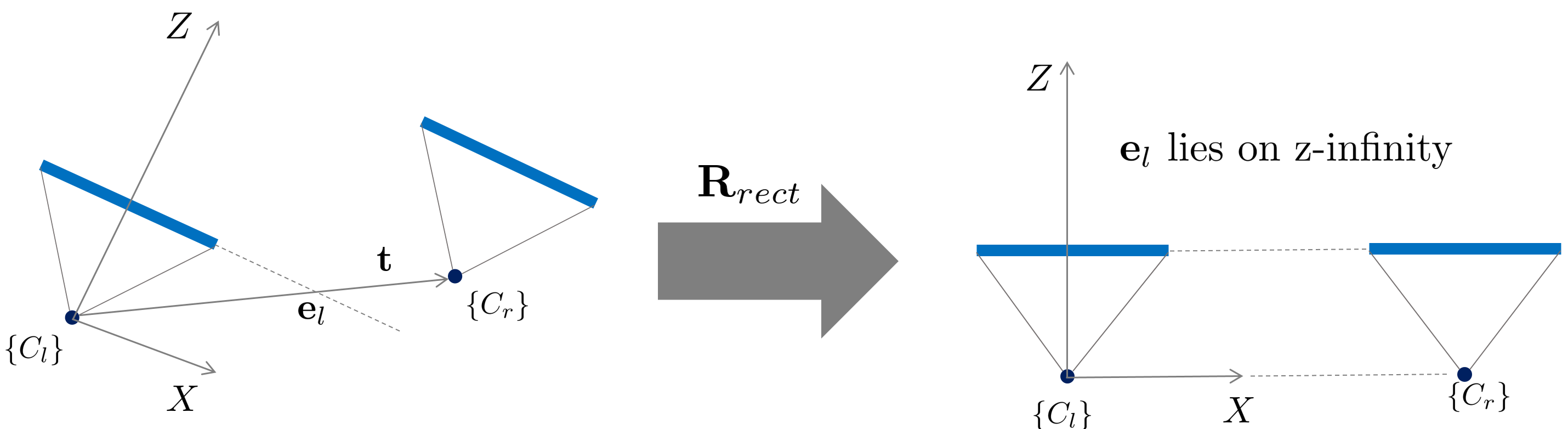
}위 함수는 앞서 구한 $\mathbf{R}, \mathbf{t}$를 사용하여 rectification matrix $\mathbf{R}_{rect}$를 구하는 함수이다. $\mathbf{t}$는 왼쪽 카메라에서 오른쪽 카메라로 방향벡터를 의미하므로 이는 곧 왼쪽 이미지 평면의 epipole $\mathbf{e}_{l}$의 방향벡터와 동일하다. rectification matrix $\mathbf{R}_{rect}$가 다음과 같을 때
$$\mathbf{R}_{rect} = \begin{bmatrix} \mathbf{r}^{\intercal}_{x} \\\mathbf{r}^{\intercal}_{y} \\ \mathbf{r}^{\intercal}_{z} \end{bmatrix}$$
각각의 열벡터 $\mathbf{r}_{x,y,z}$을 다음과 같이 설정한다.
- $\mathbf{r}_{z} = \mathbf{e}_{l} = \mathbf{t} / \| \mathbf{t} \|$ : epipole coincides with translation vector
- $\mathbf{r}_{x} = [-t_y, t_x, 0] / \sqrt{t_x^2 + t_y^2}$ : cross product of $\mathbf{e}_{l}$ and the direction vector of the optical axis
- $\mathbf{r}_{y} = \mathbf{r}_{z} \times \mathbf{r}_{x}$ : orthogonal vector
이렇게 구한 $\mathbf{R}_{rect}$는 orthogonal 성질에 의해 다음을 만족한다.
$$\mathbf{R}_{rect}\mathbf{e}_{l} = \begin{bmatrix} \mathbf{r}_{x}^{\intercal}\mathbf{e}_{l} \\ \mathbf{r}_{y}^{\intercal}\mathbf{e}_{l} \\ \mathbf{r}_{z}^{\intercal}\mathbf{e}_{l} \end{bmatrix} = \begin{bmatrix} 0 \\ 0 \\ 1 \end{bmatrix}$$
즉, $\mathbf{R}_{rect}$는 epipole을 z 무한대로 보내는 변환이다.
$\mathbf{R}_{rect}$를 구한 후 다음 공식을 사용하여 stereo rectifiication homography $\mathbf{H}_{1}, \mathbf{H}_{2}$를 구한다.
\begin{equation}
\begin{aligned}
& \mathbf{H}_{1} = \mathbf{K}\mathbf{R}_{rect}\mathbf{K}^{-1} \\
& \mathbf{H}_{2} = \mathbf{K}\mathbf{R}_{rect}\mathbf{R}^{\intercal}\mathbf{K}^{-1}
\end{aligned}
\end{equation}
Code #5
void ApplyHomography(cv::Mat &img, cv::Mat &img_out, Eigen::Matrix3d H) {
  cv::Mat _H;
  cv::eigen2cv(H, _H);

  cv::warpPerspective(img, img_out, _H,
                      cv::Size(img.size().width * 4, img.size().height * 2));
}
이미지에 homography를 적용하는 함수이다. eigen 라이브러리를 통해 구한 homography $\mathbf{H}$를 opencv 타입으로 변경한 다음 이미지에 적용한다.
Code #6
int main() {
  std::string fn_left = util::GetProjectPath() + "/picture/left.jpg";
  std::string fn_right = util::GetProjectPath() + "/picture/right.jpg";

  cv::Mat img_left = cv::imread(fn_left, 1);
  cv::Mat img_right = cv::imread(fn_right, 1);

  Eigen::MatrixXd x1_best(8, 3);
  Eigen::MatrixXd x2_best(8, 3);

  x1_best <<
	    2201.606,  421.487, 1,
        2491.521, 1233.741, 1,
        2202.928, 294.5618, 1,
        1596.858, 621.5378, 1,
        2203.898,  1175.88, 1,
        2503.346,  1275.17, 1,
        2132.505, 298.8192, 1,
        2561.777, 745.0586, 1;

	x2_best <<
		 2404.31,  533.2378, 1,
         2403.97,  1370.911, 1,
        2450.759,  408.9355, 1,
        1749.202,  654.4105, 1,
        2140.022,  1267.529, 1,
        2399.647,   1413.43, 1,
         2380.94,  405.7941, 1,
        2653.428,  899.0267, 1;


  // load intrinsic parameter.
  Eigen::Matrix3d K;
  K << 2211.75963080077, 0, 2018.81623699895,
	   0,2218.36683671952, 1120.37532022008,
	   0, 0, 1;


  Eigen::Matrix3d F;
  F = CalculateFundamentalMatrix(x1_best, x2_best);

  DrawEpipolarLines(img_left, img_right, x1_best, x2_best, F);

  Eigen::Matrix3d R;
  Eigen::Vector3d t;

  std::tie(R, t) = DecomposeFundamentalMatrix(K, F, x1_best, x2_best);

  Eigen::Matrix3d H1;
  Eigen::Matrix3d H2;
  std::tie(H1, H2) = ComputeStereoHomography(R, t, K);

  cv::Mat img_left_warped, img_right_warped;
  ApplyHomography(img_left, img_left_warped, H1);
  ApplyHomography(img_right, img_right_warped, H2);

  cv::resize(img_left_warped, img_left_warped, cv::Size(), 0.25, 0.25);
  cv::resize(img_right_warped, img_right_warped, cv::Size(), 0.25, 0.25);
  cv::imshow("warped left", img_left_warped);
  cv::imshow("warped right", img_right_warped);
  cv::moveWindow("warped left", 0, 600);
  cv::moveWindow("warped right", 1000, 600);
  cv::waitKey(0);

  return 0;
}
두 이미지를 입력으로 받은 후 미리 계산한 대응점 쌍을 x1_best, x2_best 변수에 넣는다. 또한 zhang's method를 통해 구한 카메라 내부 파라미터 $\mathbf{K}$ 또한 입력해준다. 그리고 앞서 설명한 CalculateFundamentalMatrix 함수를 통해 fundamental matrix $\mathbf{F}$를 구하고 이를 DecomposeFundamentalMatrix 함수를 통해 분해하여 $\mathbf{R}, \mathbf{t}$를 구한다. 최종적으로 ComputeStereoHomography 함수를 통해 rectification homograpy $\mathbf{H}_{1}, \mathbf{H}_{2}$를 구하여 이미지에 적용함으로써 stereo rectified된 이미지를 얻는다.
ROS-based Stereo Camera Calibration
본 섹션에서는 실제 모노카메라 2개를 결합하여 스테레오 카메라를 방법에 대해 설명한다. 본 포스트는 공부 목적으로 작성되었기 때문에 디테일한 세팅 방법은 제외하고 큰 틀에서 stereo calibration을 수행하는 방법에 대해서 설명한다. stereo calibration의 자세한 과정은 아래와 같다(출처).

우선 모노카메라 2개를 준비한다. 이 때, 두 카메라의 촬영 타이밍을 동기화해줘야 하는데 이러한 trigger를 지원하는 카메라를 구매해야 한다. internal trigger, external trigger를 지원하는 머신비전 카메라를 추천한다. (e.g., Pointgrey) 또한 external trigger를 구동하기 위한 아두이노를 1개 준비한다. 다음으로 두 카메라를 고정하기 위한 지그를 제작해야 한다. 카메라를 고정하는 다양한 지그가 있지만 필자는 알루미늄 지그를 사용하였다. 알루미늄 지그 위에 두 모노카메라를 같은 방향을 보면서 원하는 baseline 길이만큼 떨어뜨려준다. 자세한 모습은 다음과 같다.

Time Synchronization
두 대의 카메라를 동시에 사용하는 경우 disparity map을 계산하면 전방 물체에 대한 depth를 추정할 수 있다. 이를 위해 두 카메라의 이미지 획득 과정이 동기화되어야 한다. 동기화가 제대로 되지 않은 경우에는 잘못된 disparity map 계산으로 인해 부정확한 depth가 계산되며 이는 곧 부정확한 SLAM 성능으로 이어진다. 이러한 이유로 반드시 두 카메라의 촬영 타이밍을 동기화해야 한다. 따라서 촬영 타이밍 동기화 기능을 지원하는 머신비전 카메라를 구입해야 한다. 촬영 타이밍을 카메라 자체에서 지원하는 경우 internal trigger, 외부 신호를 받아서 작동하는 경우를 external trigger라고 한다. 자세한 내용은 머신비전 카메라에서 지원하는 technical document를 읽어보고 진행하면 된다.
External Trigger
아두이노를 external trigger로 사용하기 위해서는 GPIO 핀이 연결될 수 있는 배선이 필요하다. 아두이노에서 원하는 촬영 주기로 HIGH, LOW 신호를 전송하면 카메라는 해당하는 주기대로 영상을 촬영한다. 필자가 사용한 아두이노 external trigger 코드는 다음과 같다.
// 아두이노의 3번 핀 사용
int pin=3;

// 초기 설정 함수
void setup() {
    // 아두이노의 baud rate을 115200으로 설정. (단위: bit per second)
    // 간단한 데이터 전송이므로 baud rate의 크기는 자유롭게 설정 가능.
	Serial.begin(115200);
	// 3번 핀을 신호를 전송하는 핀으로 설정
	pinMode(pin, OUTPUT);
}

// 루프 함수
void loop() {
  // 30 [ms] (33 [Hz]) 주기로 LOW, HIGH 신호를 교차적으로 3번핀으로 전송
  digitalWrite(pin, LOW);
  delay(30);  // ms
  digitalWrite(pin, HIGH);
}
trigger를 사용하여 두 카메라가 동시에 촬영을 하는지 테스트하려면 카메라의 ros time이 left, right 동일한지 (<1ms) 체크하거나 ms 수준까지 측정가능한 스탑워치를 촬영하여 left, right 영상 모두 동일한 초를 촬영하였는지 체크하는 방식으로 검증한다.
ROS-based Stereo Rectification
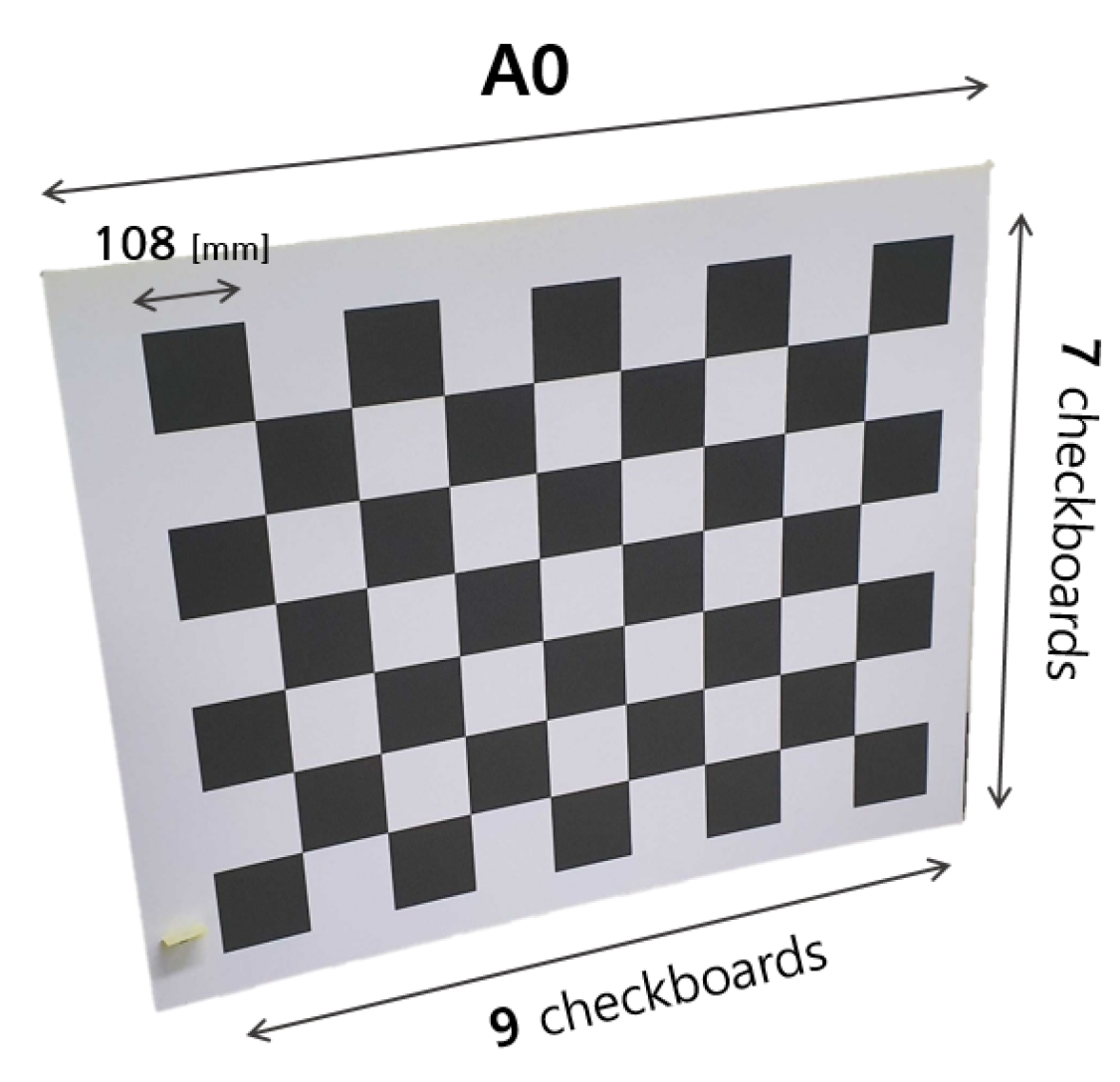
다음으로 zhang's method를 사용하여 두 카메라의 calibration paramter를 구한다. 체크보드를 실제 크기와 동일하게 인쇄한 후 평평한 면에 붙여서 고정시킨다. baseline 길이에 따라 체크보드의 크기는 적절하게 선택한다. baseline이 길수록 스트레오 카메라 자체의 크기가 커지므로 보다 정확한 calibration 이미지 취득을 위해서는 큰 크기의 체크보드가 필요하다. 예제에서는 단일 체크무늬 크기가 108 [mm]인 7x9 체크보드를 사용하였다.
다음으로 ros를 사용하여 stereo calibration을 진행한다. 다음과 같이 image_pipeline 패키지를 다운받은 후 프로그램을 빌드한다.
# clone image_pipeline repository for camera calibration package.
$ cd ~/catkin_ws/src
$ git clone https://github.com/ros-perception/image_pipeline
$ cd ~/catkin_ws && catkin_make

# update package list.
$ source  ~/catkin_ws/devel/setup.bash && rospack profile

# run streo camera calibration toolkit.
$ rosrun camera_calibration cameracalibrator.py --size 6x8 --square 0.108 right:=/camera/right/image_raw left:=/camera/left/image_raw left_camera:=/camera/left right_camera:=/camera/right  --no-service-check --approximate=0.001
정상적으로 rosrun이 실행되면 아래와 같은 calibration 화면이 나타난다.

카메라를 다양한 곳에 위치시키면서 우측 상단에 X, Y, Size, Skew 파라미터가 충족될 때까지 충분한 이미지를 확보한다. 이미지가 충분히 확보되면 CALIBRATE 버튼이 활성화되는데 이 때 해당 버튼을 클릭하면 내부적으로 opencv calibration 함수를 사용하여 스테레오 카메라의 내부, 외부 파라미터를 계산한다. 계산된 파라미터는 SAVE 버튼을 클릭하여 yaml 파일로 저장할 수 있다. yaml 파일은 다음과 같이 구성되어 있다.
 image_width: 1280
 image_height: 1024
 camera_name: left_cam
 camera_matrix:
   rows: 3
   cols: 3
   data: [889.8602805117614, 0.0, 671.07531787367, 0.0, 890.2580943164184, 531.9750294763282, 0.0, 0.0, 1.0]       8 distortion_model: plumb_bob
 distortion_coefficients:
   rows: 1
   cols: 5
   data: [-0.3105702475008413, 0.08466956187389453, 0.00011705409670444742, 0.0002672768180225955, 0.0]
 rectification_matrix:
   rows: 3
   cols: 3
   data: [1.0, 0.0, 0.0, 0.0, 1.0, 0.0, 0.0, 0.0, 1.0]
 projection_matrix:
   rows: 3
   cols: 4
   data: [716.5624389648438, 0.0, 688.0083251516589, 0.0, 0.0, 785.5123901367188, 538.0618494199916, 0.0, 0.0, 0.    0, 1.0, 0.0]
이미지의 크기(image_width, image_height 변수)와 카메라의 이름(camera name), 내부 파라미터 $\mathbf{K}$ (camera_matrix), distortion 관련 파라미터 $k_1, k_2, p_1, p_2$ (distortion_coefficients), $\mathbf{R}_{rect}$ (rectification matrix), 그리고 rectification projection matrix $\mathbf{P}_{rect} = \mathbf{K}[\mathbf{R}_{rect} | \mathbf{t}]$ (projection_matrix)가 저장되어 있다.
이 중 $\mathbf{P}_{rect}$가 실제로 rectification에 사용되는 행렬이며 left, right 카메라의 값이 서로 다르다. $\mathbf{P}^l_{rect}$를 왼쪽 카메라, $\mathbf{P}^r_{rect}$을 오른쪽 카메라의 projection matrix라고 하면 자세한 값은 다음과 같다.
$$\mathbf{P}^l_{rect} = \begin{bmatrix} f' & 0 & c'_x & 0 \\ 0 & f' & c'_y & 0 \\ 0 & 0 & 1 & 0 \end{bmatrix}$$
$$\mathbf{P}^r_{rect} = \begin{bmatrix} f' & 0 & c'_x & t_x f' \\ 0 & f' & c'_y & 0 \\ 0 & 0 & 1 & 0 \end{bmatrix}$$
$f', c'_x, c'_y$는 stereo rectified가 수행된 이후의 새로운 내부 파라미터를 의미하며 왼쪽 카메라는 원점이라고 가정하므로 마지막 열이 모두 0이고 오른쪽 카메라는 baseline만큼 x축으로 떨어져 있다고 가정하여 $t_x f'$의 값을 가진다. 위 두 $\mathbf{P}^l_{rect}, \mathbf{P}^r_{rect}$를 각각의 카메라에 적용하면 stereo rectified된 영상을 얻을 수 있다.
References
- 13.1 Stereo Rectification - Carnegie Mellon University
- Understand and Apply Stereo Rectification for Depth Maps (Part 2)
- ROS/OpenCV Stereo Calibration yaml files
'Engineering' 카테고리의 다른 글
| [SLAM] ROVIO 논문 및 코드 리뷰 (+ IEKF) (0) | 2024.01.27 |
|---|---|
| [SLAM] VINS-mono 논문 리뷰 (+ IMU preintegration) (11) | 2022.10.15 |
| [MVG] Scene Plane-based Homography 예제코드 및 설명 (C++) (0) | 2022.07.07 |
| [MVG] Vanishing Point-based Metric Rectification 예제코드 및 설명 (C++) (0) | 2022.07.03 |
| [MVG] Zhang's Calibration 예제코드 및 설명 (C++) (0) | 2022.06.29 |


