 A L I D A
해당 내용은 공부 목적으로 작성된 글입니다.
잘못된 부분이나 수정할 부분이 있다면 댓글이나 메일로 알려주시면 확인 후 수정하도록 하겠습니다.
본 포스트는 MVG part2 에서 설명한 "Computing given the homography induced by a plane" 부분을 활용하여 homography와 fundamental matrix를 구하는 내용에 대해 리뷰한다. 예제 코드는 우분투 18.04 환경에서 테스트하였으며 cmake 3.16, opencv 4.2, eigen 3.3.7 버전을 사용하여 정상적으로 작동하는 것을 확인하였다. 예제 코드는 링크를 클릭하여 다운로드하면 된다.
Scene Plane-based Homography
Input Image Setup
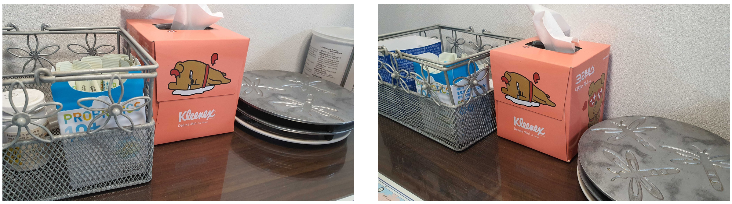
실제 월드 상에서 평면이 존재하는 물체를 촬영한다. 본 포스팅에서는 휴지케이스의 앞면을 평면으로 가정하여 촬영하였으며 촬영에 사용된 카메라의 lens distortion은 없다고 가정하였다. 평면에 존재하는 4개의 점과 평면에 존재하지 않는 2개의 점의 픽셀 좌표를 알고 있다고 가정한다. 위 사진에서 6개의 점은 다음과 같이 사용하였다.
파란색 점은 동일한 평면 위에 있는 4개의 점을 의미하고 노란색 점은 평면 위에 있지 않은 임의의 점을 의미한다.
Computing given the homography induced by a plane
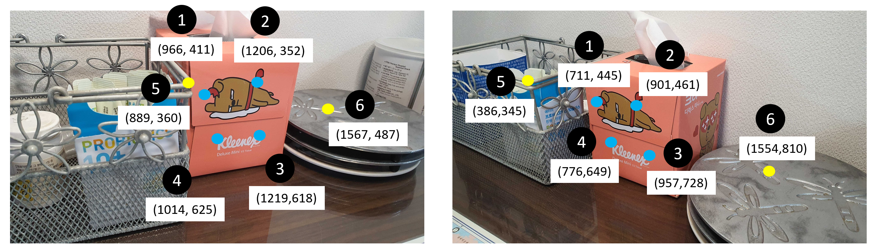
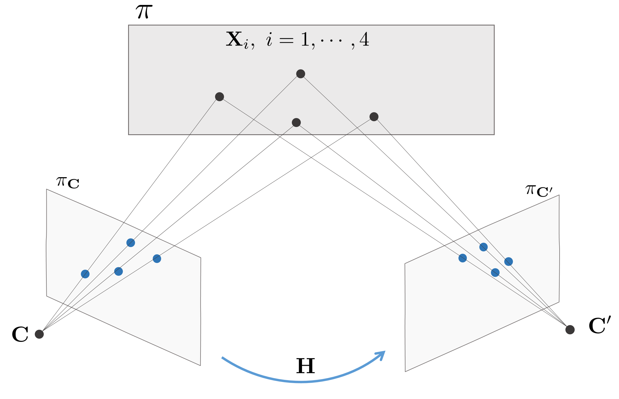
일반적으로 두 개의 카메라 행렬 대응쌍 $(\mathbf{P},\mathbf{P}^{\prime})$에 대한 Fundamental Matrix $\mathbf{F}$를 계산하기 위해서는 최소 8개의 대응점 쌍 $(\mathbf{x}_{i},\mathbf{x}_{i}^{\prime}), \ i=1,\cdots,8$이 필요하다. 하지만 Scene Plane Homography를 이용하면 6개의 대응점 쌍만 사용해도 $\mathbf{F}$를 계산할 수 있다. 단, 6개의 대응점 쌍들 중 4개 대응점 쌍 $(\mathbf{x}_{i}, \mathbf{x}_{i}^{\prime}), \ i=1,\cdots,4$에 해당하는 월드 상의 점들의 동일한 평면 $\pi$ 위에 존재해야 한다는 제약조건이 있다.
6개의 대응점 쌍으로 Fundmaental Matrix $\mathbf{F}$를 계산하는 알고리즘의 순서는 다음과 같다.
1. 월드 상의 평면 $\pi$ 위에 존재하는 4개의 점들 $\mathbf{X}_{i},\ i=1,\cdots,4$를 프로젝션한 대응점 쌍들 $(\mathbf{x}_{i}, \mathbf{x}_{i}^{\prime}), \ i=1,\cdots,4$를 사용하여 $\mathbf{x}_{i}^{\prime} = \mathbf{H}\mathbf{x}_{i}$를 만족하는 Homorgaphy $\mathbf{H}$를 계산한다. 이 때 4쌍의 대응점은 Homography $\mathbf{H}$를 유일하게 결정한다.
2. 남은 2개의 대응점 쌍 $(\mathbf{x}_{i}, \mathbf{x}_{i}^{\prime}),\ i=5,6$을 사용하여 Epipole $\mathbf{e}^{\prime}$를 구한다. $\mathbf{x}_{5}$를 Homography 변환한 $\mathbf{Hx}_{5}$와 $\mathbf{x}_{5}^{\prime}$를 사용하여 두 점을 잇는 직선을 $(\mathbf{Hx}_{5})\times \mathbf{x}_{5}^{\prime}$와 같이 구한다. $\mathbf{x}_{6}$에 대해서도 마찬가지로 적용하여 직선 $(\mathbf{Hx}_{6})\times \mathbf{x}_{6}^{\prime}$를 구한 다음 두 직선이 교차하는 점을 구하면 그 점이 곧 Epipole $\mathbf{e}^{\prime}$가 된다.
\begin{equation}
\begin{aligned}
\mathbf{e}^{\prime} = (\mathbf{Hx}_{5}) \times \mathbf{x}_{5}^{\prime} \cap (\mathbf{Hx}_{6}) \times \mathbf{x}_{6}^{\prime}
\end{aligned}
\end{equation}
3. Fundamental Matrix $\mathbf{F}$를 $\mathbf{F}=\mathbf{e}^{\prime\wedge}\mathbf{H}$를 통해 구한다.
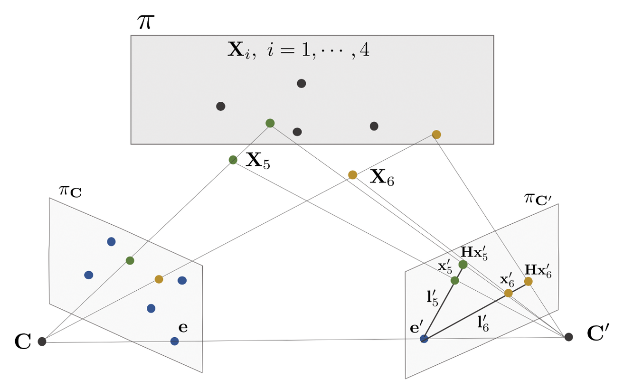
위 공식을 사용하여 $\mathbf{F}$를 계산한 후 epipolar line을 그려보면 다음과 같다.
Code Review
예제 코드는 링크를 클릭하여 다운로드하면 된다. 전체 코드는 다음과 같다.
#include "util.h"

#include <Eigen/Dense>

#include <opencv2/core/core.hpp>
#include <opencv2/core/eigen.hpp>
#include <opencv2/highgui/highgui.hpp>
#include <opencv2/opencv.hpp>

#include <iostream>
#include <string>
#include <vector>
#include <numeric>

using namespace std;

Eigen::Matrix3d ComputeHomographyDLT(Eigen::MatrixXd x1, Eigen::MatrixXd x2){
	double x1_mean_x  = x1.col(0).mean();
	double x1_mean_y  = x1.col(1).mean();
	Eigen::Vector2d centroid1;
	centroid1 << x1_mean_x, x1_mean_y;

	double x2_mean_x  = x2.col(0).mean();
	double x2_mean_y  = x2.col(1).mean();
	Eigen::Vector2d centroid2;
	centroid2 << x2_mean_x, x2_mean_y;

	// compute H1norm
	vector<double> dist1;
	for(int i=0; i<x1.rows(); i++){
		double d = std::sqrt((x1(i, 0) - centroid1(0)) * (x1(i, 0) - centroid1(0)) +
							 (x1(i, 1) - centroid1(1)) * (x1(i, 1) - centroid1(1)));
		dist1.push_back(d);
	}

	double mean_dist1 = std::accumulate(dist1.begin(), dist1.end(), 0) / dist1.size();

	Eigen::Matrix3d H1norm;
	H1norm << 1/std::sqrt(2) / mean_dist1, 0, -centroid1(0) / std::sqrt(2) / mean_dist1,
		   0, 1/std::sqrt(2) / mean_dist1, -centroid1(1) / std::sqrt(2) / mean_dist1,
		   0, 0, 1;

	// compute H2norm
	vector<double> dist2;
	for(int i=0; i<x2.rows(); i++){
		double d = std::sqrt((x2(i, 0) - centroid2(0)) * (x2(i, 0) - centroid2(0)) +
							 (x2(i, 1) - centroid2(1)) * (x2(i, 1) - centroid2(1)));
		dist2.push_back(d);
	}

	double mean_dist2 = std::accumulate(dist2.begin(), dist2.end(), 0) / dist2.size();

	Eigen::Matrix3d H2norm;
	H2norm << 1/std::sqrt(2) / mean_dist2, 0, -centroid2(0) / std::sqrt(2) / mean_dist2,
		   0, 1/std::sqrt(2) / mean_dist2, -centroid2(1) / std::sqrt(2) / mean_dist2,
		   0, 0, 1;

	x1 = (H1norm * x1.transpose()).transpose();
	x2 = (H2norm * x2.transpose()).transpose();

	Eigen::MatrixXd A(8, 9);
	for(int i=0; i<4; i++){
		double x = x1.row(i)(0);
		double y = x1.row(i)(1);
		double u = x2.row(i)(0);
		double v = x2.row(i)(1);

		Eigen::Matrix<double, 9, 1> a1,a2;
		a1 << -x, -y, -1, 0, 0, 0, u*x, u*y, u;
		a2 << 0, 0, 0, -x, -y, -1, v*x, v*y, v;


		int k = 2*i;
		A.row(k) = a1.transpose();
		A.row(k+1) = a2.transpose();
	}

	Eigen::JacobiSVD<Eigen::MatrixXd> svd(A, Eigen::ComputeFullU | Eigen::ComputeFullV);
	Eigen::MatrixXd V = svd.matrixV();
	Eigen::Matrix<double, 9 , 1> h = V.col(V.cols() - 1);

	Eigen::Matrix3d H;
	H << h(0), h(1), h(2),
	  h(3), h(4), h(5),
	  h(6), h(7), h(8);


	return H2norm.inverse() * H * H1norm;
}

void DrawEpipolarLines(cv::Mat img_left, cv::Mat img_right, Eigen::MatrixXd x1,
                       Eigen::MatrixXd x2, Eigen::Matrix3d F) {

  std::vector<cv::Scalar> colors;
  colors.push_back(cv::Scalar(255, 0, 0));
  colors.push_back(cv::Scalar(0, 255, 0));
  colors.push_back(cv::Scalar(0, 0, 255));
  colors.push_back(cv::Scalar(255, 255, 0));
  colors.push_back(cv::Scalar(255, 0, 255));
  colors.push_back(cv::Scalar(0, 255, 255));
  colors.push_back(cv::Scalar(125, 125, 0));
  colors.push_back(cv::Scalar(125, 0, 125));

  const int pt1 = -5000;
  const int pt2 = +5000;

  for (int i = 0; i < x1.rows(); i++) {
    Eigen::Vector3d x2_vec = x2.row(i);
    Eigen::Vector3d epipolar_line_left = F.transpose() * x2_vec;
    double a_l = epipolar_line_left(0);
    double b_l = epipolar_line_left(1);
    double c_l = epipolar_line_left(2);
    cv::Point2f pt_l1(pt1, (-a_l * pt1 - c_l) / b_l);
    cv::Point2f pt_l2(pt2, (-a_l * pt2 - c_l) / b_l);

    Eigen::Vector3d x1_vec = x1.row(i);
    Eigen::Vector3d epipolar_line_right = F * x1_vec;
    double a_r = epipolar_line_right(0);
    double b_r = epipolar_line_right(1);
    double c_r = epipolar_line_right(2);
    cv::Point2f pt_r1(pt1, (-a_r * pt1 - c_r) / b_r);
    cv::Point2f pt_r2(pt2, (-a_r * pt2 - c_r) / b_r);

#if 0
    std::cout << "Left" << std::endl;
    std::cout << a_l << ", " << b_l << ", " << c_l << std::endl;
    std::cout << pt_l1 << ", " << pt_l2 << std::endl;
    std::cout << "Right" << std::endl;
    std::cout << a_r << ", " << b_r << ", " << c_r << std::endl;
    std::cout << pt_r1 << ", " << pt_r2 << std::endl;
    std::cout << "-------------------------------------------------" << std::endl;
#endif
    cv::circle(img_left, cv::Point(x1_vec(0), x1_vec(1)), 20, colors[i],
               cv::FILLED, 8, 0);
    cv::circle(img_right, cv::Point(x2_vec(0), x2_vec(1)), 20, colors[i],
               cv::FILLED, 8, 0);
    cv::line(img_left, pt_l1, pt_l2, colors[i], 2);
    cv::line(img_right, pt_r1, pt_r2, colors[i], 2);
  }

  std::cout << "F\n" << F.matrix() << std::endl;

#if 1
  cv::resize(img_left, img_left, cv::Size(), 0.5, 0.5);
  cv::resize(img_right, img_right, cv::Size(), 0.5, 0.5);
  cv::imshow("epi_left", img_left);
  cv::imshow("epi_right", img_right);
  cv::moveWindow("epi_right", 1000, 0);
  cv::waitKey(0);
#endif
}


int main(){
	std::string fn_left =
		util::GetProjectPath() + "/picture/left.jpg";
	std::string fn_right =
		util::GetProjectPath() + "/picture/right.jpg";

	cv::Mat img_left = cv::imread(fn_left, 1);
	cv::Mat img_right = cv::imread(fn_right, 1);


	Eigen::Matrix<double, 4, 3> x_left, x_right;
	x_left << 966, 411, 1,
		   1206, 352, 1,
		   1219, 618, 1,
		   1014, 625, 1;
	x_right << 711, 445, 1,
			901, 461, 1,
			957, 728, 1,
			776, 649, 1;

	Eigen::Matrix3d H;

	H = ComputeHomographyDLT(x_left, x_right);

	Eigen::Vector3d x5_left, x5_right, x6_left, x6_right;
	x5_left << 889, 360, 1;
	x5_right << 386, 345, 1;
	x6_left << 1567, 487, 1;
	x6_right << 1554, 810, 1;

	Eigen::Vector3d Hx5_left = H * x5_left;
	Hx5_left = Hx5_left / Hx5_left.norm();

	Eigen::Vector3d Hx6_left = H * x6_left;
	Hx6_left = Hx6_left / Hx6_left.norm();

	Eigen::Vector3d l5, l6;

	l5 = Hx5_left.cross(x5_right);
	l6 = Hx6_left.cross(x6_right);

	Eigen::Vector3d e_r;
	e_r = l5.cross(l6);

	Eigen::Matrix3d skew_e_r;
	skew_e_r << 0, -e_r(2), e_r(1),
			 e_r(2), 0, -e_r(0),
			 -e_r(1), e_r(0), 0;

	Eigen::Matrix3d F;
	F = skew_e_r * H;

	DrawEpipolarLines(img_left, img_right, x_left, x_right, F);

}
DrawEpipolarLines() 함수는 이름 그대로 이미지에 epipolar line을 그려주는 함수이다. 해당 함수에 대한 자세한 설명은 생략한다.
How to run
본 예제코드는 cmake 프로젝트로 작성하였으며 Ubuntu 18.04, cmake 3.16, opencv 4.2, eigen 3.3.7 버전에서 정상 작동하는 것을 확인하였다. 다음 순서로 프로그램을 빌드 및 실행하면 된다.
# clone the repository
$ git clone https://github.com/gyubeomim/mvg-example
$ cd mvg-example/scene-plane-based-homography

# cmake build
$ mkdir build
$ cd build
$ cmake ..
$ make

# run example
$ ./scene
Code #1
int main(){
	std::string fn_left =
		util::GetProjectPath() + "/picture/left.jpg";
	std::string fn_right =
		util::GetProjectPath() + "/picture/right.jpg";

	cv::Mat img_left = cv::imread(fn_left, 1);
	cv::Mat img_right = cv::imread(fn_right, 1);


	Eigen::Matrix<double, 4, 3> x_left, x_right;
	x_left << 966, 411, 1,
		   1206, 352, 1,
		   1219, 618, 1,
		   1014, 625, 1;
	x_right << 711, 445, 1,
			901, 461, 1,
			957, 728, 1,
			776, 649, 1;

	Eigen::Matrix3d H;

	H = ComputeHomographyDLT(x_left, x_right);
예제 이미지 2장을 불러온다. 다음으로 이미 알고 있다고 가정한 동일 평면 상 4개의 점의 픽셀 좌표를 각각 x_left, x_right 변수에 넣어준다. 다음으로 4개의 대응점 쌍을 사용하여 homography $\mathbf{H}$를 계산한다.
Code #2
Eigen::Matrix3d ComputeHomographyDLT(Eigen::MatrixXd x1, Eigen::MatrixXd x2){
	double x1_mean_x  = x1.col(0).mean();
	double x1_mean_y  = x1.col(1).mean();
	Eigen::Vector2d centroid1;
	centroid1 << x1_mean_x, x1_mean_y;

	double x2_mean_x  = x2.col(0).mean();
	double x2_mean_y  = x2.col(1).mean();
	Eigen::Vector2d centroid2;
	centroid2 << x2_mean_x, x2_mean_y;

	// compute H1norm
	vector<double> dist1;
	for(int i=0; i<x1.rows(); i++){
		double d = std::sqrt((x1(i, 0) - centroid1(0)) * (x1(i, 0) - centroid1(0)) +
							 (x1(i, 1) - centroid1(1)) * (x1(i, 1) - centroid1(1)));
		dist1.push_back(d);
	}

	double mean_dist1 = std::accumulate(dist1.begin(), dist1.end(), 0) / dist1.size();

	Eigen::Matrix3d H1norm;
	H1norm << 1/std::sqrt(2) / mean_dist1, 0, -centroid1(0) / std::sqrt(2) / mean_dist1,
		   0, 1/std::sqrt(2) / mean_dist1, -centroid1(1) / std::sqrt(2) / mean_dist1,
		   0, 0, 1;

	// compute H2norm
	vector<double> dist2;
	for(int i=0; i<x2.rows(); i++){
		double d = std::sqrt((x2(i, 0) - centroid2(0)) * (x2(i, 0) - centroid2(0)) +
							 (x2(i, 1) - centroid2(1)) * (x2(i, 1) - centroid2(1)));
		dist2.push_back(d);
	}

	double mean_dist2 = std::accumulate(dist2.begin(), dist2.end(), 0) / dist2.size();

	Eigen::Matrix3d H2norm;
	H2norm << 1/std::sqrt(2) / mean_dist2, 0, -centroid2(0) / std::sqrt(2) / mean_dist2,
		   0, 1/std::sqrt(2) / mean_dist2, -centroid2(1) / std::sqrt(2) / mean_dist2,
		   0, 0, 1;

	x1 = (H1norm * x1.transpose()).transpose();
	x2 = (H2norm * x2.transpose()).transpose();

	Eigen::MatrixXd A(8, 9);
	for(int i=0; i<4; i++){
		double x = x1.row(i)(0);
		double y = x1.row(i)(1);
		double u = x2.row(i)(0);
		double v = x2.row(i)(1);

		Eigen::Matrix<double, 9, 1> a1,a2;
		a1 << -x, -y, -1, 0, 0, 0, u*x, u*y, u;
		a2 << 0, 0, 0, -x, -y, -1, v*x, v*y, v;


		int k = 2*i;
		A.row(k) = a1.transpose();
		A.row(k+1) = a2.transpose();
	}

	Eigen::JacobiSVD<Eigen::MatrixXd> svd(A, Eigen::ComputeFullU | Eigen::ComputeFullV);
	Eigen::MatrixXd V = svd.matrixV();
	Eigen::Matrix<double, 9 , 1> h = V.col(V.cols() - 1);

	Eigen::Matrix3d H;
	H << h(0), h(1), h(2),
	  h(3), h(4), h(5),
	  h(6), h(7), h(8);


	return H2norm.inverse() * H * H1norm;
}
4개의 대응점 쌍을 사용하여 homography $\mathbf{H}$를 계산한다. 이 때, 행렬 $\mathbf{H}$는 주어진 대응점쌍 $\mathbf{x} \leftrightarrow \mathbf{x}^{\prime}$으로 구성된 행렬이므로 대응점쌍들을 정규화(normalization)하지 않고 바로 해를 구하는 경우 $\mathbf{x}_{i} = (x>>1, y>>1, 1)$과 같이 마지막 값에 비해서 처음 두 값의 크기가 매우 크게 되므로 수치적으로 불안정한 문제를 가진다. 따라서 $\mathbf{x}_{i}, \mathbf{x}_{i}^{\prime}$를 Centroid가 0이고 Centroid로부터 평균거리가 $\sqrt{2}$가 되도록하는 Homography 변환 $\mathbf{H}_{1}, \mathbf{H}_{2}$를 적용한다 (H1norm, H2norm 변수).
\begin{equation}
\begin{aligned}
& \mathbf{x}_{i} \leftarrow \mathbf{H}_{1}\mathbf{x}_{i} \\
& \mathbf{x}_{i}^{\prime} \leftarrow \mathbf{H}_{2} \mathbf{x}_{i}^{\prime} \\
\end{aligned}
\end{equation}
위 과정은 코드 상에서 x1 = (H1norm * x1.transpose()).transpose(); x2 = (H2norm * x2.transpose()).transpose(); 과정과 동일하다. 이렇게 변환된 대응쌍점들을 사용하여 수치적으로 안정적인 homography $\mathbf{H}^{\prime}$ 계산할 수 있다. $\mathbf{H}'$은 다음 공식을 만족한다.
$$\mathbf{x}'_{i} = \mathbf{H}'\mathbf{x}_{i}$$
$$\begin{bmatrix} u_{i} \\ v_{i} \\ 1 \end{bmatrix} = \begin{bmatrix} h_1 & h_2 & h_3 \\ h_4 & h_5 & h_6 \\ h_7 & h_8 & h_9 \end{bmatrix} \begin{bmatrix} x_{i} \\ y_{i} \\ 1 \end{bmatrix}$$
따라서 $\mathbf{x}'_{i} \times \mathbf{H}'\mathbf{x}_{i} = 0$이 성립하고 이를 $\mathbf{A}\mathbf{h} = 0$의 Direct Linear Transform (DLT) 형태로 변경하면 다음과 같다.
$$\begin{bmatrix} -x_i& -y_i& -1& 0&0&0& u_i x_i & u_i y_i &u_i \\ 0&0&0&-x_i&-y_i&-1&v_i x_i&v_i y_i & v_i \end{bmatrix} \begin{bmatrix} h_1 \\ h_2 \\ \vdots \\ h_9 \end{bmatrix} = 0$$
- $\mathbf{h} = \begin{bmatrix} h_1 & h_2 & \dots & h_9 \end{bmatrix}^{\intercal}$
위 선형시스템의 null space를 구하면 이는 곧 $\mathbf{h}$의 해가 된다. 이를 통해 $\mathbf{H}'$를 구할 수 있다. 이와 같이 $\mathbf{H}^{\prime}$를 계산한 다음 다시 원래의 대응점쌍 $\mathbf{x} \leftrightarrow \mathbf{x}^{\prime}$으로 복원하기 위해
\begin{equation}
\begin{aligned}
0 & = (\mathbf{H}_{2}\mathbf{x}^{\prime})^{\intercal}\mathbf{H}^{\prime}(\mathbf{H}_{1}\mathbf{x}) \\
& = \mathbf{x}^{\intercal}(\mathbf{H}_{2}^{\intercal} \mathbf{H}^{\prime}\mathbf{H}_{1})\mathbf{x}
\end{aligned}
\end{equation}
처럼 $\mathbf{H} = \mathbf{H}_{2}^{\intercal} \mathbf{H}^{\prime}\mathbf{H}_{1}$를 통해 원래 대응점쌍의 homography $\mathbf{H}$를 계산할 수 있다. 이는 return H2norm.inverse() * H * H1norm; 구문과 같다.
Code #3
	Eigen::Vector3d x5_left, x5_right, x6_left, x6_right;
	x5_left << 889, 360, 1;
	x5_right << 386, 345, 1;
	x6_left << 1567, 487, 1;
	x6_right << 1554, 810, 1;

	Eigen::Vector3d Hx5_left = H * x5_left;
	Hx5_left = Hx5_left / Hx5_left.norm();

	Eigen::Vector3d Hx6_left = H * x6_left;
	Hx6_left = Hx6_left / Hx6_left.norm();

	Eigen::Vector3d l5, l6;

	l5 = Hx5_left.cross(x5_right);
	l6 = Hx6_left.cross(x6_right);

	Eigen::Vector3d e_r;
	e_r = l5.cross(l6);

	Eigen::Matrix3d skew_e_r;
	skew_e_r << 0, -e_r(2), e_r(1),
			 e_r(2), 0, -e_r(0),
			 -e_r(1), e_r(0), 0;

	Eigen::Matrix3d F;
	F = skew_e_r * H;

	DrawEpipolarLines(img_left, img_right, x_left, x_right, F);

}
다음으로 $\mathbf{x}_{5}, \mathbf{x}_{6}$의 픽셀 좌표를 입력하고 이를 통해 epipole $\mathbf{e}'$를 구해야 한다. $\mathbf{x}_{5}$를 Homography 변환한 $\mathbf{Hx}_{5}$와 $\mathbf{x}_{5}^{\prime}$를 사용하여 두 점을 잇는 직선을 $(\mathbf{Hx}_{5})\times \mathbf{x}_{5}^{\prime}$와 같이 구한다(l5, l6 변수). $\mathbf{x}_{6}$에 대해서도 마찬가지로 적용하여 직선 $(\mathbf{Hx}_{6})\times \mathbf{x}_{6}^{\prime}$를 구한 다음 두 직선이 교차하는 점을 구하면 그 점이 곧 Epipole $\mathbf{e}^{\prime}$가 된다(e_r 변수).
\begin{equation}
\begin{aligned}
\mathbf{e}^{\prime} = (\mathbf{Hx}_{5}) \times \mathbf{x}_{5}^{\prime} \cap (\mathbf{Hx}_{6}) \times \mathbf{x}_{6}^{\prime}
\end{aligned}
\end{equation}
최종적으로 fundamental Matrix $\mathbf{F}$ $\mathbf{F}=\mathbf{e}^{\prime\wedge}\mathbf{H}$를 통해 구한다(F 변수). $\mathbf{F}$를 통해 epipolar line을 그릴 수 있고 이를 이미지에 표현하면 다음과 같다.
'Engineering' 카테고리의 다른 글
| [SLAM] VINS-mono 논문 리뷰 (+ IMU preintegration) (11) | 2022.10.15 |
|---|---|
| [MVG] Stereo Camera Calibration 예제코드 및 설명 (C++) (3) | 2022.07.14 |
| [MVG] Vanishing Point-based Metric Rectification 예제코드 및 설명 (C++) (0) | 2022.07.03 |
| [MVG] Zhang's Calibration 예제코드 및 설명 (C++) (0) | 2022.06.29 |
| [MVG] Affine & Metric Rectification 예제코드 및 설명 (C++) (0) | 2022.06.22 |


