 A L I D A
1. Introduction to ROVIO
ROVIO는 RObust Visual Inertial Odometry의 약자로 ETHZ의 ASL 연구실의 Bloesch et al.이 제안한 VIO 알고리즘이다. IROS 학회에 2015년에 처음 발표되었으며 이후 IJRR에 2017년 자세한 설명을 포함한 저널이 게재되었다. ROVIO는 MSCKF와 더불어 대표적인 필터링 기반 Tightly-coupled VIO이다. MSCKF와 가장 큰 차이점은 밝기 오차(photometric error)를 IEKF의 Update 과정에 사용한다는 점이다. 이를 통해 실시간 성능의 가벼우면서도 모션블러 및 텍스쳐가 적은 환경에 강인한 알고리즘을 제안하였다.
1.1. Loosely-coupled VIO vs Tightly-coupled VIO

Loosely-coupled VIO는 카메라와 IMU의 센서 데이터에서 각각 pose를 추출한 후 이를 퓨전하는 방법을 말한다. Pose를 추출한 후 퓨전하기 때문에 비교적 알고리즘 구성이 단순하지만 정확도가 낮다는 단점이 있다.

이와 달리, tightly-coupled VIO는 카메라와 IMU의 센서 데이터를 모은 후 한 번에 pose를 추출하는 방법을 말한다. Tightly-coupled VIO는 pose를 구하는 구체적인 방법에 따라 필터링 방법과 최적화 방법으로 패러다임이 나뉜다. Loosely-coupled VIO에 비해 정확도가 높지만 연산량이 많다는 단점이 있다.
1.2. Filtering-based vs Optimization-based
필터링 기반(Filtering-based) 방법은 EKF를 사용하여 IMU와 카메라를 퓨전하는 방법을 말한다. 일반적으로 IMU는 prediction 스텝에 사용되고 카메라는 update 스텝에 사용된다. 대표적인 논문으로는 MSCKF(07'), ROVIO(15'), S-MSCKF(18') 등이 있으며 이 중 MSCKF는 Google Tango(16') 프로젝트에 사용되어 실제 기기에 사용되었다. 필터링 기반 방법은 최적화 기반 방법 대비 연산량이 비교적 작다는 장점이 있어 소형 임베디드 기기에 활용하기 적합하다. 하지만 incremental하게 상태를 추정하기 때문에 상대적으로 최적화 기반 방법 대비 정확도가 낮은 편이다.
최적화 기반(Optimization-based) 방법은 비선형 최적화 방법을 사용하여 IMU와 카메라를 퓨전하는 방법을 말한다. 2010년대초 IMU preintegration 기법이 개발되면서 본격적으로 최적화 기반의 VIO들이 많이 개발되었다. 대표적인 알고리즘으로는 OKVIS(15'), VINS-mono(17'), VI-DSO(18'), ORB-SLAM3(20') 등이 있다. 최적화 방법은 필터링 방식에 비해 정확도가 높은 편이지만 연산량이 상대적으로 많다는 단점이 존재한다.
1.3. Representation of 3D rotations
ROVIO에서는 물체의 회전을 표현하기 위해 SO(3)군을 사용한다. 이 때, 유의할 점은 SO(3)군이 회전 행렬이나 쿼터니언을 특정하는 것이 아닌 순수하게 두 좌표계 사이의 회전을 표현하는 집합(또는 군)을 사용한다는 것이다. 이러한 순수 회전을 의미하는 SO(3)군은 Quaternion kinematics for the error-state Kalman filter 내용 정리 포스팅의 2.2 섹션에서 자세히 설명하고 있다. 또는 저자의 다른 논문인 [5]를 참조하면 된다. 회전 행렬로 표현된 SO(3)군에 대한 설명은 리군 이론(Lie Theory) 개념 정리 포스팅의 SO(3) 섹션을 참조하면 된다.
따라서 논문에서는 $\mathbf{q}$를 사용하여 설명하고 있지만 이는 쿼터니언이 아닌 순수 SO(3) 회전군을 의미하므로 혼동하지 않도록 유의한다. $\mathbf{q} \in SO(3)$를 회전 행렬로 변환하는 연산자 $\mathbf{C}$는 다음과 같다.
\begin{equation}
\begin{aligned}
\mathbf{C}(\mathbf{q}) : SO(3) \mapsto \mathbb{R}^{3\times3}
\end{aligned}
\end{equation}
임의의 벡터 $\mathbf{r} \in \mathbb{R}^{3}$이 주어졌을 때 이를 $\mathbf{q}$만큼 회전하려면 $\mathbf{q}(\mathbf{r})$ 기호를 사용하여 표현한다. 이를 풀어쓰면 다음과 같다.
\begin{equation}
\begin{aligned}
\mathbf{q}(\mathbf{r}) \triangleq \mathbf{C}(\mathbf{q}) \mathbf{r} \in \mathbb{R}^{3}
\end{aligned}
\end{equation}
- 위 식은 복잡해보이지만 $\mathbf{q}$와 동일한 회전 크기의 $\mathbf{R}$이 있을 때 $\mathbf{Rr}$을 수행하는 것과 동일하다. 즉, $\mathbf{q}(\mathbf{r}) = \mathbf{Rr}$.
1.4. Representation of 3D unit vectors
ROVIO에서는 단위 크기를 가진 bearing vector $\mu$를 사용하기 때문에 이와 관련된 미분 방정식을 유도할 때 3D 단위 벡터의 표현법을 활용한다. IJRR 2017 저널[2]의 섹션 3.3을 보면 임의의 회전 군 $\mu \in SO(3)$에 대하여 다음 연산을 정의할 수 있다.
\begin{equation}
\begin{aligned}
& \mathbf{n}(\mu) := \mu(\mathbf{e}_z) \in S^{2} \subset \mathbb{R}^{3} \\
& \mathbf{N}(\mu) := [\mu(\mathbf{e}_x), \mu(\mathbf{e}_y)] \in \mathbb{R}^{3 \times 2}
\end{aligned}
\end{equation}
- $\mathbf{e}_{x/y/z}$ : 특정 방향(orientation) $\mu$의 각 축에 대한 basis vector
- $\mathbf{n}(\mu)$ : 특정 방향(orientation) $\mu$의 z축 벡터
- $\mathbf{N}(\mu)$ : 특정 방향(orientation) $\mu$의 x,y축 벡터 (z축과 수직인 접평면(tangent plane)를 의미)
여기서 주의할 점은 [2]의 3.3 섹션을 설명할 때는 $\mu \in SO(3)$가 회전에 대한 SO(3)군을 의미하는 반면 이후 챕터에서는 bearing vector $\mu \in \mathbb{R}^{3}$로 표현하고 있다는 점이다. [2]의 Appendix A에 (82) 공식에서 이를 활용한 유도 공식이 등장한다.

위 식에서 편미분되는 부분은 $\frac{\partial \mu}{\partial \mu}$인데 공식대로면 1이 나와야 하지만 $[\mu]_{\times} \mathbf{N}(\mu)$가 도출된다. 이는 [2]의 (32) 공식에 따른 유도 결과이다.

즉, 실제 편미분 되는 식은 $\frac{\partial \mathbf{n}(\mu)}{\partial \mu}$이다. 논문에서도 의미가 명확하면 $\mathbf{n}(\mu)$를 $\mu$로 표현한다고 명시하였으니 논문을 보면서 헷갈리지 않도록 유의해야 한다.

1.5. Robocentric representation

ROVIO의 저자는 fully robocentric 표현법을 사용하여 시스템의 상태를 표현한 것이 논문의 핵심 contribution이라고 하였다. Robocentric 표현법이란 IMU의 위치, 속도, 특징점의 좌표를 월드 좌표계 $\{\mathcal{I}\}$에서 본 값으로 표현하는 것이 아닌 관측된 그 좌표계 그대로 사용하는 것을 의미한다. IMU에서 위치 추정하는 상황을 예로 들어보자.
World-centric
IMU 측정값이 들어오면 이를 통해 위치의 증분량을 계산한 후 월드 좌표계로 변환하는 연산 $\mathbf{q}_{\mathcal{I}\mathcal{B}}$을 적용하여 $_\mathcal{I} \mathbf{r}_{\mathcal{I} \mathcal{B}}$ 파라미터를 추정한다.
Robocentric
IMU 측정값이 들어오면 $_\mathcal{B} \mathbf{r}_{\mathcal{I} \mathcal{B}}$를 사용하여 파라미터를 추정한다. 이는 별도의 월드 좌표계로 변환하는 비선형 연산 $\mathbf{q}_{\mathcal{I}\mathcal{B}} \cdot \ _\mathcal{B} \mathbf{r}_{\mathcal{I} \mathcal{B}}$를 수행하지 않기 때문에 연산량이 감소하고 선형성 측면에서도 좋기 때문에 정확도가 증가하는 장점이 있다.
특징점에 대한 bearing vector $\mu$와 역깊이(inverse depth) $\rho$ 또한 카메라 좌표계 $\{\mathcal{C}\}$를 그대로 사용한다. $\mu, \rho$도 동일하게 카메라 $\rightarrow$ IMU $\rightarrow$ 월드 좌표계로 변환해야 하는 비선형 연산이 없으므로 선형성이 증가되어 정확도가 증가하고 관측 가능성(observability)가 증가하는 특징을 지닌다. ROVIO에서는 $\mu, \rho$에 대한 state propagation 수식을 유도하여 IEKF update 스텝을 통해 업데이트할 수 있게 되었는데 이 또한 ROVIO의 핵심 contribution 중 하나이다. 자세한 내용은 해당 섹션를 참조하면 된다.
1.6. Bearing vector and inverse depth
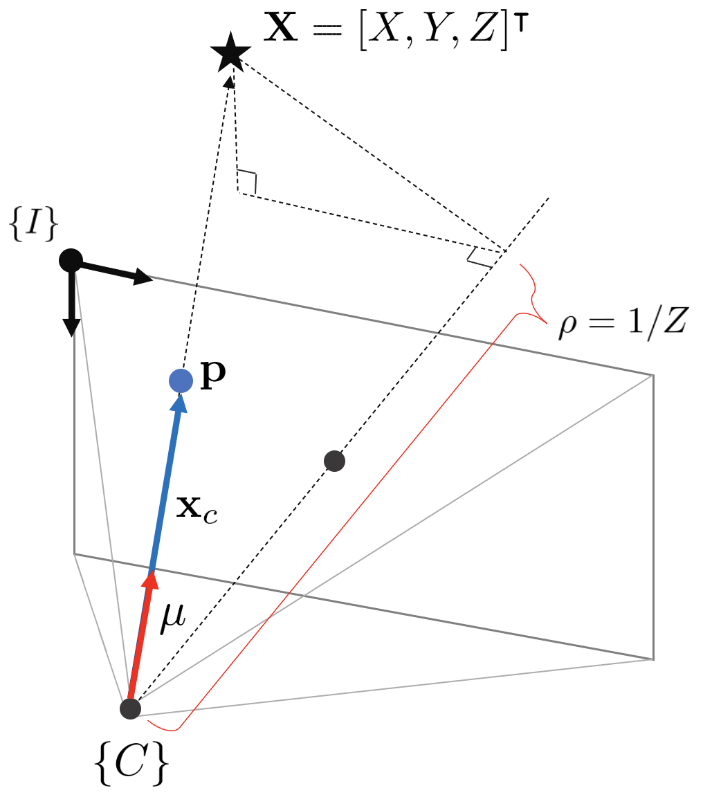
ROVIO에서는 3차원 공간 상의 점 $\mathbf{X}$를 표현할 때 카메라의 중심 좌표계 $\{C\}$로부터 표현한 bearing vector $\mu$와 역깊이 $\rho=1/Z$를 사용하여 표현한다. 이 때, $\mu$는 크기가 1인 단위 벡터이다. 단위벡터 $\mu$를 사용하면 파라미터를 추정할 때 안정적으로 추정할 수 있으며, 역깊이 $\rho$ 또한 멀리 떨어진 점일수록 0에 가까운 값을 지니게 되어 IEKF가 발산하지 않고 안정적으로 추정할 수 있도록 해준다.
$\mathbf{x}_{c}$는 카메라 좌표계 $\{C\}$에서 이미지 평면 상의 점 $\mathbf{p}$까지 벡터를 의미할 때, $\mathbf{X}, \mathbf{x}_{c}, \mathbf{p}, \mu$ 사이의 변환 관계는 다음과 같다.
\begin{equation}
\begin{aligned}
& \mathbf{X} \mapsto \mathbf{x}_{c} \quad : \quad \begin{bmatrix} X \\ Y \\ Z \end{bmatrix} \mapsto \begin{bmatrix} X/Z \\ Y/Z \\ 1 \end{bmatrix}
\end{aligned}
\end{equation} \begin{equation}
\begin{aligned}
& \mathbf{x}_{c} \mapsto \mathbf{p} \quad : \quad \begin{bmatrix} X/Z \\ Y/Z \\ 1 \end{bmatrix} \mapsto \frac{1}{Z} \begin{bmatrix} f_x X + c_{x} \\ f_y Y + c_{y} \end{bmatrix}
\end{aligned}
\end{equation} \begin{equation}
\begin{aligned} \mathbf{p} \mapsto \mathbf{x}_{c} \quad : \quad \begin{bmatrix} u \\ v \end{bmatrix} \mapsto \begin{bmatrix} \frac{u-c_x}{f_x} \\ \frac{v-c_y}{f_y} \\ 1\end{bmatrix}
\end{aligned}
\end{equation} \begin{equation}
\begin{aligned}
& \mathbf{x}_{c} \mapsto \mu \quad : \quad \mathbf{x}_{c} \mapsto \frac{\mathbf{x}_{c}}{\left \| \mathbf{x}_{c} \right\|}
\end{aligned}
\end{equation} \begin{equation}
\begin{aligned}
\mu \mapsto \mathbf{x}_{c} \quad : \quad \begin{bmatrix} \mu_{x} \\ \mu_{y} \\ \mu_{z} \end{bmatrix} \mapsto \begin{bmatrix} \mu_{x} / \mu_{z} \\ \mu_ {y} / \mu_{z} \\ 1 \end{bmatrix}
\end{aligned}
\end{equation}
- $f_x, f_y, c_x, c_y$ : 카메라 내부(intrinsic) 파라미터
역깊이 $\rho$를 통해 깊이를 구하는 함수를 $d(\rho)$라고 정의한다.
\begin{equation}
\begin{aligned}
d(\rho) = 1/\rho
\end{aligned}
\end{equation}
임의의 3차원 공간 상의 점 $\mathbf{X}$는 $\mathbf{x}_{c} \cdot d(\rho)$ 로 표현할 수 있다. $\mathbf{x}_{c}$는 bearing vector $\mu$에 $\mu_{z}$를 나눠주면 구할 수 있기 때문에 ROVIO에서는 $\mathbf{x}_{c}$라는 용어를 별도로 사용하지 않고 $\mu$로 표기하고 있는 것으로 보인다.
\begin{equation}
\begin{aligned}
\mathbf{X} = \mu \cdot d(\rho)
\end{aligned}
\end{equation}
이미지 좌표계 $\{I\}$로부터 표현한 픽셀 좌표 $\mathbf{p}$가 주어졌을 때 $\mathbf{p}$와 $\mu$ 사이의 변환 관계는 다음과 같다.
\begin{equation}
\begin{aligned}
& \mathbf{p} = \pi(\mu) \\
& \mu \mapsto \mathbf{p} : \begin{bmatrix} \mu_{x} \\ \mu_{y} \\ \mu_{z} \end{bmatrix} \mapsto \frac{1}{Z} \begin{bmatrix} f_{x} (\mu_{x} / \mu_{z}) + c_{x} \\ f_{y} (\mu_{y}/ \mu_{z}) + c_{y} \end{bmatrix}
\end{aligned}
\end{equation}
2. Multilevel patches and photometric error
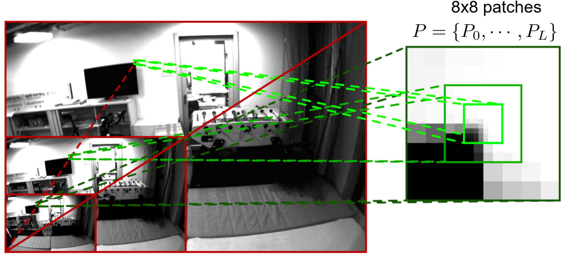
ROVIO는 피라미드 이미지에서 패치를 추출하여 동일한 패치 크기(6x6 또는 8x8)에서도 다양한 영역의 정보를 포함할 수 있도록 하였다. 이미지 패치를 사용하여 순차적인 이미지 사이의 밝기 오차(photometric error)를 innovation term으로 설정하였다.
2.1. Photometric error
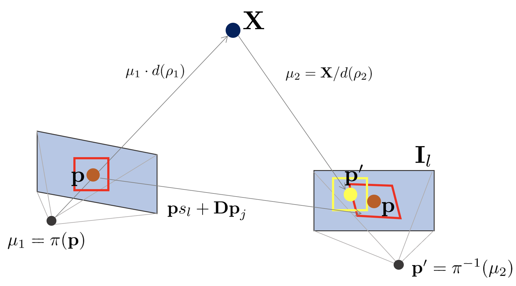
l 번째 피라미드 이미지에서 패치의 j번째 점에 대한 밝기 오차 $e_{l,j}$는 다음과 같이 정의한다.
\begin{equation}
\begin{aligned}
e_{l,j}(\mathbf{p}, P,I,\mathbf{D}) = P_{l}(\mathbf{p}_{j}) - aI_{l}(\mathbf{p}s_{l}+\mathbf{Dp}_{j}) - b
\end{aligned}
\end{equation}
- $\mathbf{P}_{l}(\mathbf{p}_{j})$ : 이미지 패치 중 j번째 점의 예측된 밝기값 (노란색 정사각형), IEKF에서 $h(\mathbf{x}^{-}_{k}, n_{k})$에 해당
- $\mathbf{I}_{l}(\mathbf{p}s_{l} + \mathbf{Dp}_{j})$ : 이미지 패치 중 j번째 점의 관측된 밝기값 (빨간색 일그러진 사각형), IEKF에서 $\mathbf{z}_{t}$에 해당
- $s_{l} = 0.5^{l}$ : 피라미드 스케일 파라미터
- $a, b$ : affine brightness 파라미터. 이미지 패치의 평균 밝기값에 기초하여 값이 변경된다.
위 그림에서 왼쪽 이미지는 t-1 시간의 이미지이고 오른쪽 이미지는 t 시간의 이미지라고 하자. t-1 이미지에서 특징점 $\mathbf{p}$가 주어졌고 이를 중심으로 6x6 이미지 패치가 있다고 가정하자. t 시간에 IEKF prediction 스텝에 의해 $\mu_{1}, \rho_{1}$이 $\mu_{2}, \rho_{2}$로 업데이트되어 특징점이 $\mathbf{p}$에서 $\mathbf{p}'$로 변경되어 빨간색 정사각형은 노란색 정사각형으로 변하게 된다. 이는 IEKF update 스텝의 예측값으로 사용된다. 다음으로 선형변환행렬(linear warping matrix) $\mathbf{D}$에 의해 특징점의 위치 $\mathbf{p}$는 변하지 않지만 주변의 패치가 빨간색 정사각형에서 빨간색 일그러진 사각형으로 모양이 변형된다. 이는 IEKF update 스텝의 관측값으로 사용된다.
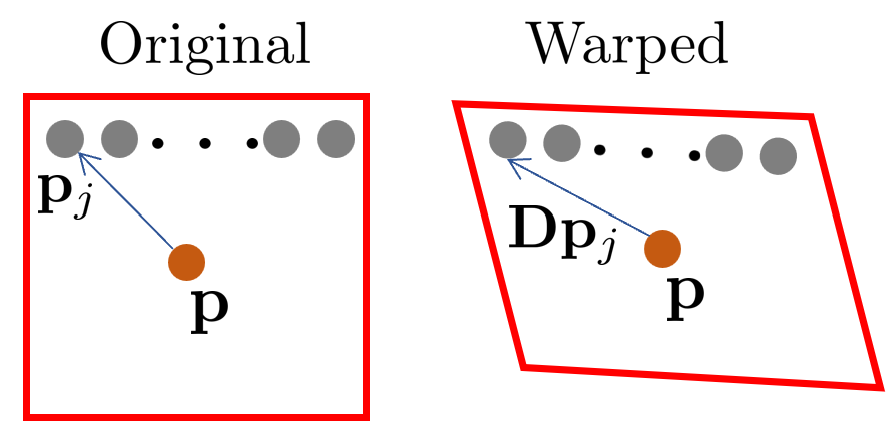
$\mathbf{D}$는 다음과 같다. $\mathbf{D}\mathbf{p}_{j}$는 $\mu_{1} \rightarrow \mu_{2}$ 변환 관계를 고려하여 정사각형이 아닌 변형(warped)된 형태의 이미지 패치를 참조하는 형태가 된다.
\begin{equation}
\begin{aligned}
\mathbf{D} = \frac{\partial \pi(\mu_{2})}{\partial \mu_{2}} \frac{\partial f(\mu_{1})}{\partial \mu_{1}} \frac{\partial \pi^{-1}(\mathbf{p}_{1})}{\partial \mathbf{p}_{1}} \in \mathbb{R}^{2\times2}
\end{aligned}
\end{equation}
$e_{l,j} (\mathbf{p},P,I,\mathbf{D})$는 l번째 피라미드 이미지의 이미지 패치 중 j번째 점에 대한 밝기 오차를 의미한다. 따라서 이를 모든 피라미드와 모든 이미지 패치에 대한 에러로 표현하면 $\mathbf{b}(\mathbf{p},P,I,\mathbf{D})$ 같은 벡터가 된다. 미세한 픽셀 위치 변화량 $\delta \mathbf{p}$이 더해진 $\mathbf{b}$는 다음과 같이 테일러 1차 근사를 통해 표현할 수 있다.
\begin{equation}
\begin{aligned}
\mathbf{b}(\hat{\mathbf{p}} + \delta \mathbf{p}, P,I,\mathbf{D}) \simeq \mathbf{b}(\hat{\mathbf{p}}, P,I,\mathbf{D}) + \mathbf{A}(\hat{\mathbf{p}},I,\mathbf{D})\delta \mathbf{p}
\end{aligned}
\end{equation}
- $\mathbf{A}(\hat{\mathbf{p}}, I, \mathbf{D})$ : $\frac{\partial \mathbf{b}(\hat{\mathbf{p}}, P,I,\mathbf{D}) }{\partial \delta \mathbf{p}}$ 자코비안 행렬
- $\delta \mathbf{p}$ : 미세한 픽셀 위치 변화량
$\delta \mathbf{p}$의 최적해는 GN(Gauss-Newton)방법을 통해 다음과 같이 구할 수 있다.
\begin{equation} \label{eq:1}
\begin{aligned}
\mathbf{A}(\hat{\mathbf{p}},I,\mathbf{D})^{\intercal}\mathbf{A}(\hat{\mathbf{p}},I,\mathbf{D})\delta \mathbf{p} = -\mathbf{A}(\hat{\mathbf{p}},I,\mathbf{D})^{\intercal}\mathbf{b}(\hat{\mathbf{p}}, P,I,\mathbf{D})
\end{aligned}
\end{equation}
$\mathbf{A}(\hat{\mathbf{p}},I,\mathbf{D})^{\intercal}\mathbf{A}(\hat{\mathbf{p}},I,\mathbf{D})$의 역행렬을 구하여 오른쪽 식으로 넘기면 최적의 해 $\delta \mathbf{p}^{*}$를 구할 수 있다.
2.2. QR decomposition of $\mathbf{A}$ matrix
자코비안 행렬 $\mathbf{A}$는 특징점의 개수, 피라미드 레벨에 따라 크기가 변하는 행렬이다. 예를 들어 이미지 패치 크기가 6x6이고 특징점 10개를 트래킹하고 있으며 피라미드 레벨이 4까지 있다면 $\mathbf{A}$의 크기는 6x6x10x4 --> (1440 x 1440)의 크기를 가진다. $\mathbf{A}$ 행렬의 크기가 클수록 IEKF의 속도가 기하급수적으로 느려지기 때문에 가능한한 행렬의 크기를 줄여야 하는데 ROVIO 논문에서는 $\mathbf{A}$ 행렬에 QR 분해를 사용함으로써 행렬의 크기를 줄이는 방법을 사용하였다.
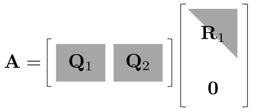
QR 분해는 임의의 행렬을 직교(orthogonal) 행렬 $\mathbf{Q}$와 상삼각행렬 $\mathbf{R}$로 분해하는 방법을 말한다. 이 때, $\mathbf{A}$가 정사각행렬인 경우 $\mathbf{R}$ 행렬은 모든 값이 0인 행이 존재하지 않지만 $\mathbf{A}$가 직사각행렬이면 $\mathbf{R}$은 모든 값이 0인 행을 포함한다. 자코비안 행렬 $\mathbf{A}$는 일반적으로 overdetermined system이므로 행이 열보다 긴 (아래로 긴) 직사각형 행렬의 형태를 지닌다. 따라서 이를 QR분해하면 $\mathbf{R} = [ \mathbf{R}_{1}, \mathbf{0}]^{\intercal}$이 된다.
\begin{equation}
\begin{aligned}
\mathbf{A}(\mathbf{p}_{i},I,\mathbf{D}) &= \mathbf{Q}(\mathbf{p}_{i}, I,\mathbf{D}_{i}) \mathbf{R}(\mathbf{p}_{i}, I, \mathbf{D}) \\
& = \begin{bmatrix} \mathbf{Q}_{1}(\mathbf{p}_{i}, I,\mathbf{D}_{i}) & \mathbf{Q}_{2}(\mathbf{p}_{i}, I,\mathbf{D}_{i}) \end{bmatrix} \begin{bmatrix} \mathbf{R}_{1}(\mathbf{p}_{i}, I, \mathbf{D}) \\ \mathbf{0} \end{bmatrix}
\end{aligned}
\end{equation}
따라서 위와 같이 블록 행렬 곱에 의해 $\mathbf{A}$ 행렬은 $\mathbf{Q}_{1}\mathbf{R}_{1}$ 행렬로 축소된다. 이를 기존 식에 대입하면 다음과 같다.
\begin{equation}
\begin{aligned}
& \mathbf{b}(\hat{\mathbf{p}} + \delta \mathbf{p}, P,I,\mathbf{D}) \simeq \mathbf{b}(\hat{\mathbf{p}}, P,I,\mathbf{D}) + \mathbf{A}(\hat{\mathbf{p}},I,\mathbf{D})\delta \mathbf{p} \\
& \rightarrow \mathbf{b}(\hat{\mathbf{p}} + \delta \mathbf{p}, P,I,\mathbf{D}) \simeq \mathbf{b}(\hat{\mathbf{p}}, P,I,\mathbf{D}) + \mathbf{Q}_{1}(\hat{\mathbf{p}}, I,\mathbf{D}_{i}) \mathbf{R}_{1}(\hat{\mathbf{p}}, I, \mathbf{D}) \delta \mathbf{p}
\end{aligned}
\end{equation}
이후 양 변에 $\mathbf{Q}_{1}^{\intercal}$을 곱하면 최종적으로 다음과 같은 식이 얻어진다. ($\mathbf{Q}_{1}^{\intercal}\mathbf{Q}_{1} = \mathbf{I}$)
\begin{equation}
\begin{aligned}
\rightarrow\mathbf{Q}_{1}^{\intercal}(\hat{\mathbf{p}}, I,\mathbf{D}_{i}) \mathbf{b}(\hat{\mathbf{p}} + \delta \mathbf{p}, P,I,\mathbf{D}) \simeq \mathbf{Q}_{1}^{\intercal}(\hat{\mathbf{p}}, I,\mathbf{D}_{i}) \mathbf{b}(\hat{\mathbf{p}}, P,I,\mathbf{D}) + \mathbf{R}_{1}(\hat{\mathbf{p}}, I, \mathbf{D}) \delta \mathbf{p}
\end{aligned}
\end{equation}
ROVIO에서는 위 식을 IEKF Update 스텝의 innovation term으로 사용한다.
\begin{equation}
\boxed { \begin{aligned}
\mathbf{y}_{i,j} = \mathbf{Q}_{1}^{\intercal}(\pi(\mu^{+}_{i,j}), I,\mathbf{D}_{i}) \mathbf{b}(\pi(\mu^{+}_{i,j}), P_{i},I,\mathbf{D})
\end{aligned} }
\end{equation}
- $\mathbf{y}_{i,j}$ : i번째 IEKF update 스텝에서 j번째 iteration 수행 시 innovation term
- $\pi(\mu^{+}_{i,j}) = \mathbf{p}^{+}_{i,j}$: i번째 IEKF update 스텝에서 j번째 iteration 수행 시 bearing vector의 posterior
Innovation term의 자코비안 행렬 $\mathbf{H}$는 다음과 같다.
\begin{equation}
\boxed { \begin{aligned}
\mathbf{H}_{i,j} = \mathbf{R}_{1}(\pi(\mu^{+}_{i,j}),I,\mathbf{D}) \frac{d \pi}{d \mu}(\mu^{+}_{i,j})
\end{aligned} }
\end{equation}
3. Iterated EKF
Kalman Filter
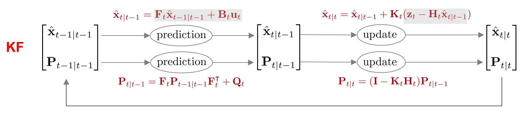
Kalman filter(KF)는 선형 동적 시스템에 대한 상태 $\mathbf{x}$와 공분산 $\mathbf{P}$의 최적값을 재귀적으로 추정하는 알고리즘이다. KF는 prediction 스텝과 update 스텝으로 구분된다. (자세한 내용은 칼만필터(Kalman Filter) 개념 정리 포스트 참조)
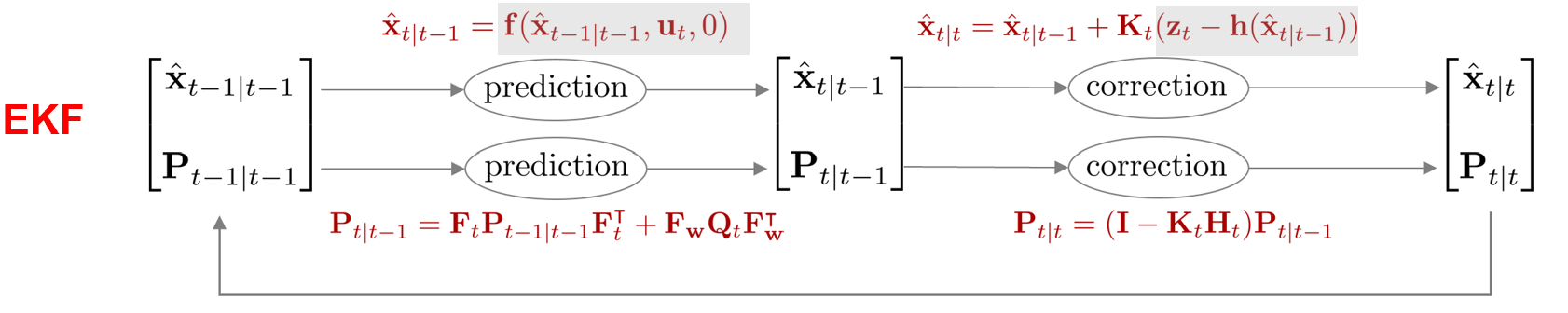
Extended Kalman Filter
만약 상태변수 $\mathbf{x}$에 비선형 항이 있다면 현재 시점에 대한 선형화(linearization)을 수행하여 KF를 수행하는 extended kalman filter(EKF)를 사용해야 한다. 문제는 EKF SLAM의 경우 선형화 과정에서 누적된 에러로 인해 시간이 지날수록 pose의 정확도가 떨어진다는 것이다. 이는 개념적으로 봤을 때 GN 최적화를 iteration=1만큼 돌린 것과 유사하다.
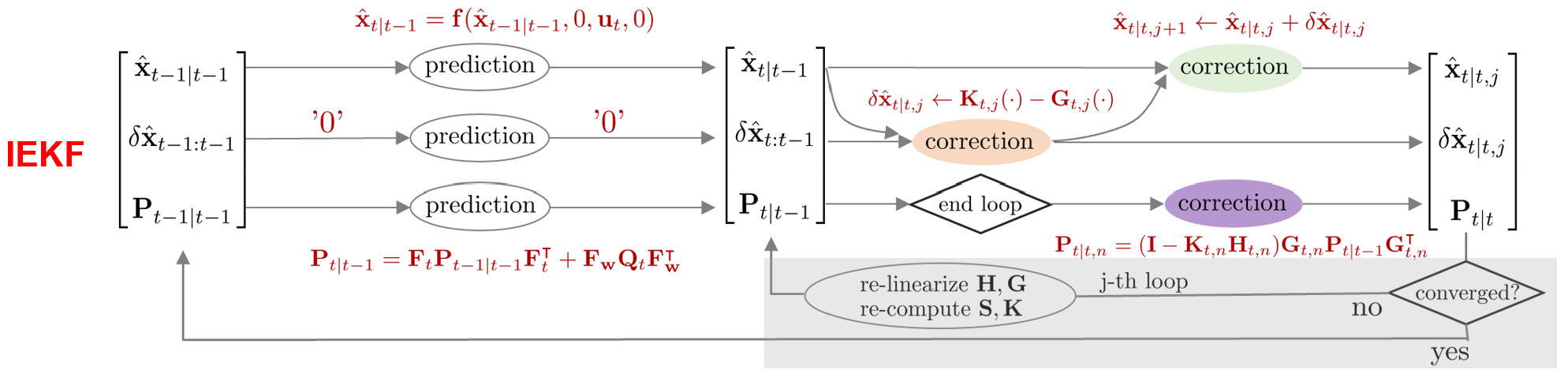
Iterated Extended Kalman Filter
Iterated EKF(IEKF)는 EKF의 선형화 오차 단점을 극복하기 위해 update 스텝에서 상태 변수 $\mathbf{x}$ 자체를 추정하는 것이 아닌 상태 변수의 변화량 $\Delta \mathbf{x}$를 반복적으로(iterative) 추정한다. 변화량 $\Delta \mathbf{x}$가 특정 값 이하로 내려가는 경우 더 이상 업데이트가 되지 않는다고 판단하고 update 스텝을 종료한다. 이는 개념적으로 GN 최적화를 iteration=n만큼 돌리는 것과 유사한 결과를 얻는다. 엄밀하게 말하면 iterated error-state kalman filter (IESKF)이지만 본 논문에서는 IEKF라고 언급하고 있으므로 본 포스팅에서도 IEKF라고 언급한다.
3.1. IEKF formulation
비선형 항을 포함한 상태변수 $\mathbf{x}$와 관측값 $\mathbf{y}$는 다음과 같이 정의할 수 있다.
\begin{equation}
\begin{aligned}
& \mathbf{x}_{k} = f(\mathbf{x}_{k-1}, w_{k-1}). \quad \cdots \text{Motion model} \\
& \mathbf{z}_{k} = h(\mathbf{x}_{k}, n_{k}) \quad \cdots \text{Measurement model}
\end{aligned}
\end{equation}
- $w \sim \mathcal{N}(0, \mathbf{W})$
- $n \sim \mathcal{N}(0, \mathbf{R})$
- $\mathbf{y}_{k} = \mathbf{z}_{k} - h(\mathbf{x}_{k}, n_{k})$ : innovation term
3.2. Prediction step
ROVIO는 IMU 입력이 들어오면 prediction 스텝을 진행한다. 일반적으로 IMU는 고속(~1000hz)로 들어오기 때문에 실시간 성능을 유지하기 위해 일정 시간동안 IMU 값들을 저장한 다음 한 번에 병합(merge)하여 처리하는 방식을 기본값으로 사용한다.
이전 k-1 스텝에서 posterior 평균과 공분산 $\mathbf{x}^{+}_{k-1}, \mathbf{P}^{+}_{k-1}$이 주어졌을 때 IEKF의 prediction 스텝은 EKF와 동일하게 현재 k 스텝의 prior 평균과 공분산 $\mathbf{x}^{-}_{k}, \mathbf{P}^{-}_{k}$를 추정한다.
\begin{equation}
\begin{aligned}
& \mathbf{x}^{-}_{k} = f(\mathbf{x}^{+}_{k-1}, 0) \\
& \mathbf{P}^{-}_{k} = \mathbf{F}_{k-1}\mathbf{P}^{+}_{k-1}\mathbf{F}_{k-1}^{\intercal} + \mathbf{G}_{k-1}\mathbf{W}_{k-1}\mathbf{G}_{k-1}^{\intercal}
\end{aligned}
\end{equation}
이 때, 자코비안 $\mathbf{F}_{k-1}, \mathbf{G}_{k-1}$은 다음과 같다.
\begin{equation}
\begin{aligned}
& \mathbf{F}_{k-1} = \frac{\partial f}{\partial \mathbf{x}_{k-1}}(\mathbf{x}^{+}_{k-1}, 0) \\
& \mathbf{G}_{k-1} = \frac{\partial f}{\partial \mathbf{w}_{k-1}}(\mathbf{x}^{+}_{k-1}, 0)
\end{aligned}
\end{equation}
3.2.1. State propagation
ROVIO에서 IEKF의 상태 변수 $\mathbf{x}$는 다음과 같이 정의된다. (N: 랜드마크의 개수)
\begin{equation}
\begin{aligned}
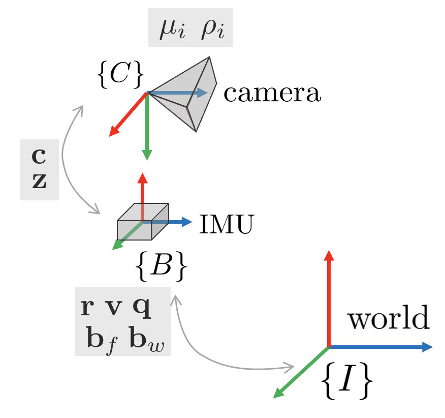
\mathbf{x} := (\mathbf{r}, \mathbf{v}, \mathbf{q}, \mathbf{b}_{f}, \mathbf{b}_{w}, \mathbf{c}, \mathbf{z}, \mu_{0}, \cdots, \mu_{N}, \rho_0, \cdots, \rho_{N})
\end{aligned}
\end{equation}
- $[\cdot]_{\times}$ : 벡터의 반대칭 행렬(skew symmetric matrix)
- $\mathbf{r} = _\mathcal{B}\mathbf{r}_{\mathbf{I}\mathcal{B}}$ : IMU 위치 (robocentric 표현)
- $\mathbf{v} = _\mathcal{B}\mathbf{v}_{\mathcal{B}}$ : IMU 속도 (robocentric 표현)
- $\mathbf{q} = \mathbf{q}_{\mathcal{I}\mathcal{B}}$ : IMU 방향 (orientation)
- $\mathbf{b}_{f}$: IMU 가속도 bias
- $\mathbf{b}_{w}$: IMU 각속도 bias
- $\mathbf{c} = _\mathcal{B}\mathbf{r}_{\mathbf{B}\mathcal{C}}$: 카메라와 IMU 사이의 상대 위치 (IMU 좌표계 기준)
- $\mathbf{z} = \mathbf{q}_{\mathcal{C}\mathcal{B}}$: 카메라와 IMU 사이의 상대 방향 (from IMU to Camera)
- $\mu_{i}$ : i번째 특징점의 bearing vector
- $\rho_{i}$ : i번째 특징점의 inverse depth
IEKF prediction 스텝의 모션 모델 $f(\cdot, \cdot)$을 유도하기 위해 각각의 변수를 미분하면 다음과 같다.
\begin{equation} \label{eq:rovio1}
\begin{aligned}
& \dot{\mathbf{r}} = -[\hat{\mathbf{w}}]_{\times}\mathbf{r} + \mathbf{v} + w_{r} \\
& \dot{\mathbf{v}} = -[\hat{\mathbf{w}}]_{\times}\mathbf{v} + \hat{\mathbf{f}} + \mathbf{q}^{-1}(\mathbf{g}) \\
& \dot{\mathbf{q}} = -\mathbf{q}(\hat{\mathbf{w}}) \\
& \dot{\mathbf{b}}_{f} = w_{bf} \\
& \dot{\mathbf{b}}_{w} = w_{bw} \\
& \dot{\mathbf{c}} = w_{c} \\
& \dot{\mathbf{z}} = w_{z} \\
& \dot{\mu}_{i} = \mathbf{N}(\mu_{i})^{\intercal} \bigg( \hat{\mathbf{w}}_{\mathcal{C}} + [\mathbf{n}(\mu_{i})]_{\times} \frac{\hat{\mathbf{v}}_{\mathcal{C}}}{d(\rho_{i})} \bigg) + w_{\mu,i} \\
& \dot{\rho_{i}} = -\mathbf{n}(\mu_{i})^{\intercal} \frac{\hat{\mathbf{v}}_{\mathcal{C}}}{d'(\rho_{i})} + w_{\rho,i}
\end{aligned}
\end{equation}
- $\hat{\mathbf{f}}$ : 실제 IMU 가속도
- $\hat{\mathbf{w}}$ : 실제 IMU 각속도
- $\hat{\mathbf{v}}_{\mathcal{C}} = \mathbf{z}(\mathbf{v} + [\hat{\mathbf{w}}]_{\times}\mathbf{c})$ : 실제 카메라의 속도
- $\hat{\mathbf{w}}_{\mathcal{C}} = \mathbf{z}(\hat{\mathbf{w}})$ : 실제 카메라의 각속도
IMU에서 측정되는 가속도 $\tilde{\mathbf{f}}$와 각속도 $\tilde{\mathbf{w}}$는 가속도 $\hat{\mathbf{f}}$와 실제 각속도 $\hat{\mathbf{w}}$에 bias와 noise가 추가된 값이다.
\begin{equation}
\begin{aligned}
& \tilde{\mathbf{f}} = \hat{\mathbf{f}} + \mathbf{b}_{f} + w_{f}. \\
& \tilde{\mathbf{w}} = \hat{\mathbf{w}} + \mathbf{b}_{w}+ w_{w}
\end{aligned}
\end{equation}
따라서 실제 가속도와 각속도는 다음과 같이 구할 수 있다.
\begin{equation}
\begin{aligned}
& \hat{\mathbf{f}} = \tilde{\mathbf{f}} - \mathbf{b}_{f} - w_{f} \\
& \hat{\mathbf{w}} = \tilde{\mathbf{w}} - \mathbf{b}_{w} - w_{w}
\end{aligned}
\end{equation}
State equation in discrete time
지금까지 유도한 식을 컴퓨터로 구현하기 위해서는 연속 시간(continuous time)을 이산 시간(discrete time)으로 변환하여 차분 방정식으로 표현해야 한다. 미분 방정식에 대한 수치 해법은 euler, midpoint, RK4 등 여러 방법이 있으나 ROVIO에서는 euler 방법을 통해 이산화하였다.
\begin{equation} \label{eq:rovio2}
\begin{aligned}
& \mathbf{r}_{k+1} = \mathbf{r}_{k} + \Delta t \cdot \mathbf{q}_{\mathcal{I}\mathcal{B}_{k}} \mathbf{v}_{\mathcal{B}_{k}} \\
& \mathbf{v}_{k+1} = (\mathbf{I} - \Delta t [\hat{\mathbf{w}}_{\mathcal{B}_{k+1}}]_{\times}) \mathbf{v}_{\mathcal{B}_{k}} + \Delta t(\hat{\mathbf{f}}_{\mathcal{I}\mathcal{B}_{k+1}} + \mathbf{q}^{-1}_{\mathcal{I}\mathcal{B}_{k}} \cdot \mathbf{g}_{\mathcal{I}}) \\
& \mathbf{q}_{k+1} = \mathbf{q}_{k} \cdot \text{Exp}(\Delta t \hat{\mathbf{w}}_{\mathcal{B}_{k+1}}) \\
& \mathbf{b}_{f,k+1} = \mathbf{b}_{f,k} + \Delta t \cdot\mathbf{w}_{f,k} \\
& \mathbf{b}_{w,k+1} = \mathbf{b}_{w,k} + \Delta t \cdot\mathbf{w}_{w,k} \\
& \mathbf{c}_{k+1} = \mathbf{c}_{k} + \Delta t \cdot\mathbf{w}_{c,k} \\
& \mathbf{z}_{k+1} = \text{Exp}(\Delta t \mathbf{w}_{z,k}) \cdot \mathbf{z}_{k} \\
& \mu_{i,k+1} = \text{Exp}\bigg( \Delta t \Big[ (\mathbf{I} - \mathbf{n}(\mu_{i,k})\mathbf{n}(\mu_{i,k})^{\intercal}) \hat{\mathbf{w}}_{\mathcal{C}} + [\mathbf{n}(\mu_{i,k})]_{\times} \frac{\hat{\mathbf{v}}_{\mathcal{C}}}{d(\rho_{i,k})} + \mathbf{N}(\mu_{k})\mathbf{w}_{\mu,i} \Big] \bigg) \otimes \mu_{i, k} \\
& \rho_{i,k+1} = \rho_{i,k} + \Delta t \mathbf{n}(\mu_{i,k})^{\intercal} \frac{\hat{\mathbf{v}}_{\mathcal{C}}}{d'(\rho_{i,k})} + \Delta t \mathbf{w}_{\rho,i}
\end{aligned}
\end{equation}
- $\text{Exp}(\mathbf{w})$ : $\mathbf{w} \in \mathbb{R}^{3}$ 벡터를 SO(3)군으로 변환하는 exponential mapping
- $\otimes$ : SO(3)군 곱셈 연산자
위 식은 ROVIO 코드 중 IMUPrediction::evalPrediction() 메소드에 구현되어 있다. 최종적으로 위 식을 통해 이전 k-1 스텝의 posterior 평균 $\mathbf{x}^{+}_{k-1}$이 주어졌을 때, 현재 k 스텝의 상태 변수 $\mathbf{x}^{-}_{k}$를 예측(predict)할 수 있다.
\begin{equation}
\begin{aligned}
\mathbf{x}^{-}_{k} = f(\mathbf{x}^{+}_{k-1}, 0)
\end{aligned}
\end{equation}
Jacobian $\mathbf{F}_{k-1}$ in discrete time
자코비안 행렬 $\mathbf{F}_{k-1}$은 다음과 같이 구할 수 있다.
\begin{equation}
\begin{aligned}
\mathbf{F}_{k-1} & = \frac{\partial f}{\partial \mathbf{x}_{k-1}}(\mathbf{x}^{+}_{k-1}, 0) \\
& = \begin{bmatrix} \mathbf{I} & \Delta t \mathbf{q}_{\mathcal{I}\mathcal{B}_{k-1}} & -\Delta t [\mathbf{q}_{\mathcal{I}\mathcal{B}_{k-1}} \mathbf{v}_{\mathcal{B}_{k-1}}]_{\times} & 0 & 0 & \cdots \\
0 & \mathbf{I} - [\Delta t \mathbf{w}_{\mathcal{B}_{k}}]_{\times} & \Delta t \mathbf{q}_{\mathcal{I}\mathcal{B}_{k-1}}^{-1}[\mathbf{g}_{\mathcal{I}}]_{\times} & - \Delta t \mathbf{I} & -\Delta t [\mathbf{v}_{\mathcal{B}_{k-1}}]_{\times} &\cdots \\
0 & 0 & \mathbf{I} & 0 & -\Delta t \mathbf{q}_{\mathcal{I}\mathcal{B}_{k-1}} \Gamma(\Delta t \mathbf{w}_{\mathcal{I}\mathcal{B}_{k}}) &\cdots \\
0 & 0 & 0 & \mathbf{I}&0 &\cdots \\
0 & 0 & 0 & 0 & \mathbf{I} & \cdots \\ \vdots & \vdots & \vdots &\vdots &\vdots & \ddots \end{bmatrix}
\end{aligned}
\end{equation}
각각의 행열마다 의미하는 상태는 다음과 같다. 이외에 $\cdots$으로 표기한 부분은 bearing vector $\mu$와 inverse depth $\rho$에 관련된 항이다.
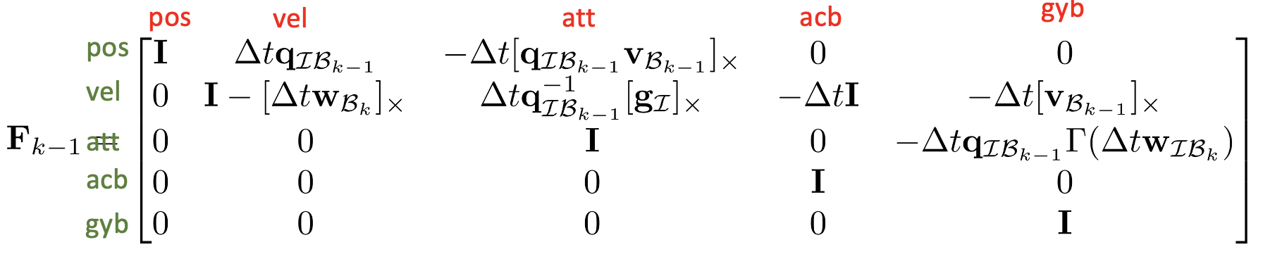
위 식은 ROVIO 코드 중 IMUPrediction::jacPreviousStateI() 메소드에 구현되어 있다.
3.3. Update step
ROVIO는 카메라에서 이미지 입력이 들어올 때마다 update 스텝을 수행한다. Prediction 스텝에 의해 propagation된 상태 변수 $\mathbf{x}^{-}_{k}$와 공분산 $\mathbf{P}^{-}_{k}$을 입력으로 사용한다. EKF의 update 스텝은 다음과 같은 최적화 문제를 푸는 것과 동일하다[4].
\begin{equation}
\begin{aligned}
\min_{\mathbf{x}^{+}_{k}} \quad \left\| \mathbf{x}^{+}_{k} \boxminus \mathbf{x}^{-}_{k} \right\|_{(\mathbf{P}^{-}_{k})^{-1}} + \left\| \mathbf{y}_{k} \right\|_{(\mathbf{J}_{k}\mathbf{R}_{k}\mathbf{J}_{k}^{\intercal})^{-1}}\end{aligned}
\end{equation}
- $\left\| \mathbf{a} \right\|_{\mathbf{B}} = \mathbf{a}^{\intercal}\mathbf{B}\mathbf{a}$ : 마할라노비스(mahalanobis) 거리
- $\mathbf{y}_{k} = \mathbf{z}_{k}-h(\mathbf{x}^{+}_{k}, 0)$ : innovation term. 앞서 photometric error를 통해 유도하였다.
EKF는 위 식을 최소화하는 $\mathbf{x}^{+}_{k}$를 한 번만 추정한다. 이와 달리 IEKF는 상태 변수의 변화량 $\Delta \mathbf{x}_{k}$를 반복적으로 추정한다. j번 반복하여 추정된 수식은 다음과 같이 나타낼 수 있다.
\begin{equation}
\begin{aligned}
\min_{\Delta \mathbf{x}_{k,j}} \quad \left\| \mathbf{x}^{+}_{k,j} \boxminus \mathbf{x}^{-}_{k} + \mathbf{L}^{-1}_{k,j} \Delta \mathbf{x}_{k,j} \right\|_{(\mathbf{P}^{-}_{k})^{-1}} + \left\| \mathbf{y}_{k,j} + \mathbf{H}_{k,j}\Delta\mathbf{x}_{k,j} \right\|_{(\mathbf{J}_{k}\mathbf{R}_{k}\mathbf{J}_{k}^{\intercal})^{-1}}
\end{aligned}
\end{equation}
- $\mathbf{L}_{k,j} = \frac{\partial (\mathbf{x}^{-}_{k} \boxplus \Delta \mathbf{x})}{\partial \Delta \mathbf{x}}(\mathbf{x}^{+}_{k,j} \boxminus \mathbf{x}^{-}_{k})$
- $\mathbf{H}_{k,j} = \frac{\partial ( \mathbf{z}_{k}-h(\mathbf{x}^{+}_{k}, 0)) }{\partial \mathbf{x}_{k}}(\mathbf{x}^{+}_{k,j},0)$
- $\mathbf{J}_{k,j} = \frac{\partial (\mathbf{z}_{k}-h(\mathbf{x}^{+}_{k}, 0)) }{\partial \mathbf{n}_{k}}(\mathbf{x}^{+}_{k,j},0)$
위 식을 미분하여 0으로 설정 후 전개하면 다음과 같은 식을 얻을 수 있다.
\begin{equation}
\begin{aligned}
& \mathbf{S}_{k,j} = \mathbf{H}_{k,j}\mathbf{L}_{k,j}\mathbf{P}^{-}_{k}\mathbf{L}_{k,j}^{\intercal}\mathbf{H}^{\intercal}_{k,j} + \mathbf{J}_{k,j}\mathbf{R}_{k}\mathbf{J}^{\intercal}_{k,j} \\
& \mathbf{K}_{k,j} = \mathbf{L}_{k,j}\mathbf{P}^{-}_{k}\mathbf{L}_{k,j}^{\intercal}\mathbf{H}^{\intercal}_{k,j}\mathbf{S}^{-1}_{k,j} \\
& \Delta\mathbf{x}_{k,j} = \mathbf{K}_{k,j}\bigg(\mathbf{H}_{k,j}\mathbf{L}_{k,j}( \mathbf{x}^{+}_{k,j} \boxminus \mathbf{x}^{-}_{k}) - \mathbf{z}_{k} - h(\mathbf{x}^{+}_{k,j},0) \bigg) - \mathbf{L}_{k,j}(\mathbf{x}^{+}_{k,j} \boxminus \mathbf{x}^{-}_{k}) \\
& \mathbf{x}^{+}_{k,j+1} = \mathbf{x}^{+}_{k,j} \boxplus \Delta\mathbf{x}_{k,j}
\end{aligned}
\end{equation}
색상을 추가하여 시각적으로 잘 보이도록 표현하면 아래와 같다.
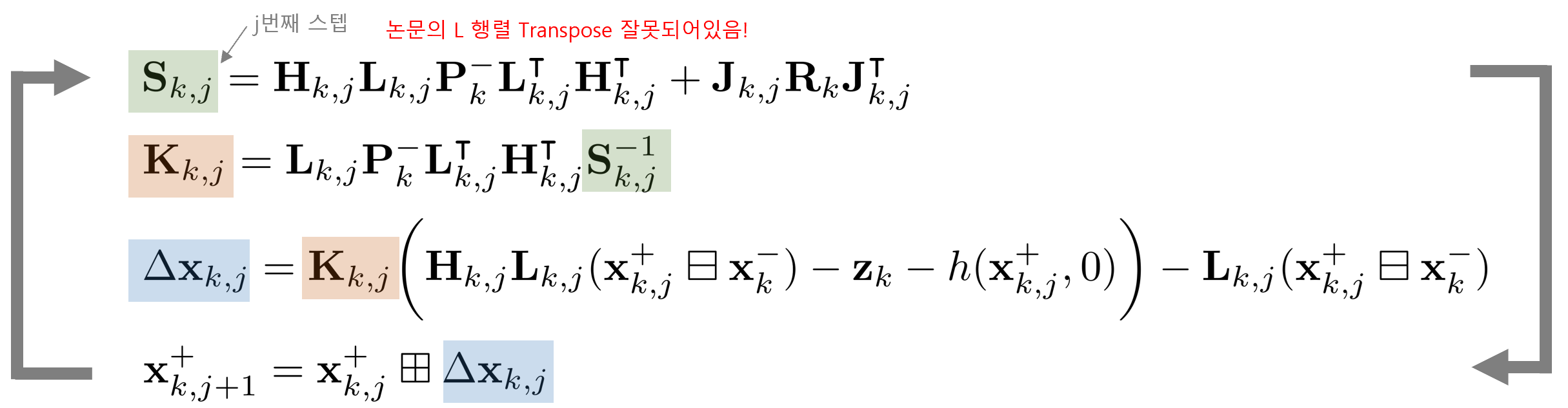
위 식을 변화량 $\Delta \mathbf{x}_{k}$가 특정 값 이하로 작아질 때까지 반복하여 기존 상태 변수에 업데이트한다. 루프를 탈출하면 posterior 공분산 $\mathbf{P}^{+}_{k}$를 계산한다.
\begin{equation}
\begin{aligned}
\mathbf{P}^{+}_{k} = (\mathbf{I} - \mathbf{K}_{k,n}\mathbf{H}_{k,n}) \mathbf{L}_{k,n}\mathbf{P}^{-}_{k}\mathbf{L}^{\intercal}_{k,n}
\end{aligned}
\end{equation}
4. Landmark management
IEKF 프레임워크는 앞서 말한 것처럼 특징점(=landmark)의 개수에 따라 연산량이 기하급수적으로 증가하기 때문에 실시간 성능을 확보하기 위해서는 특징점의 개수를 잘 관리해야 한다.
4.1. Detection and scoring
이미지 패치를 위한 특징점은 다음과 같은 과정에 의해 탐지된다.
- 새로운 이미지 패치를 위한 특징점을 추출할 때는 잘 알려진 FAST Detector를 사용한다
- 현재 트래킹하고 있는 특징점과 가까운 점들은 제거한다
- 식 ($\ref{eq:1}$)에서 $\mathbf{A}^{\intercal}\mathbf{A}$는 hessian 행렬 $\mathbf{H}$를 의미한다. $\mathbf{H}$에 대한 eigenvalue를 구해보면 $\lambda_{1}, \lambda_{2}$가 나오는데 이 값들의 크기에 따라 이미지 패치가 평면인지, 엣지인지, 코너인지 판단할 수 있다.
- \begin{equation}
\begin{aligned}
\mathbf{A}(\hat{\mathbf{p}}, I, \mathbf{D})^{\intercal}\mathbf{A}(\hat{\mathbf{p}}, I, \mathbf{D}) = \mathbf{H} \rightarrow \text{extract } (\lambda_1, \lambda_2)
\end{aligned}
\end{equation}
- Shi-Tomasi Score를 사용하여 해당 점이 평면인지, 엣지인지, 코너인지를 스코어링한다.
- 이 때, 모든 피라미드 이미지에 대해 모두 점수를 계산한다.
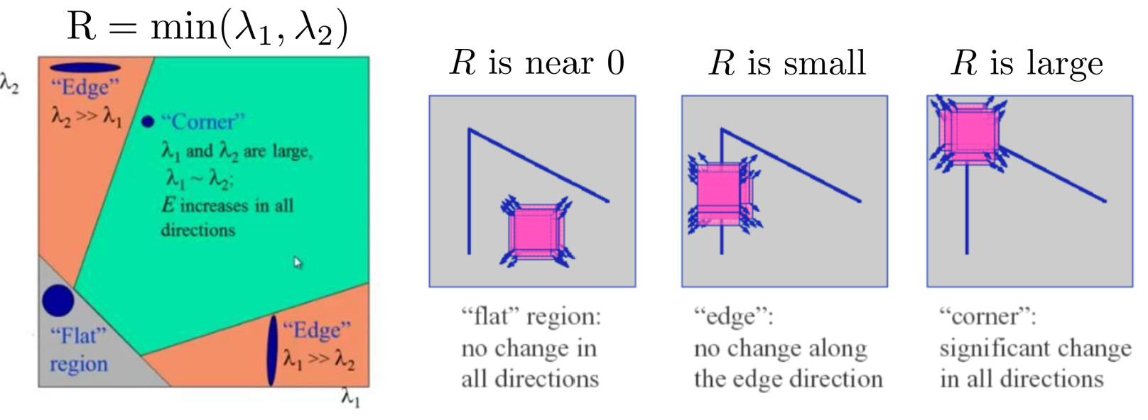
3. 과정에서 스코어를 $R = \min(\lambda_{1}, \lambda_{2})$로 잡으면 둘 중 가장 작은 eigenvalue가 선정되고 이 값의 크기에 따라 위 그림과 같이 평면, 엣지, 코너를 판별할 수 있다. ROVIO는 이 중 코너인 점들을 추출하여 특징점의 개수를 관리하였다.
4.2. Tracking and pruning
특징점은 탐지하는 과정 뿐만 아니라 탐지된 이후에도 지속적으로 트래킹할 것인지 여부를 결정한다.
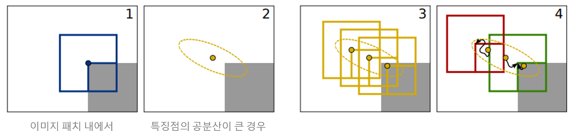
-
트래킹하고 있는 특징점의 공분산이 큰 경우 (e.g., 방금 탐지된 특징점), 한 패치 내에서 여러 점들을 동시에 트래킹한다. 공분산 ellipse 내에 있는 여러 점들을 동시에 IEKF Update 과정을 통해 반복적으로 업데이트한다
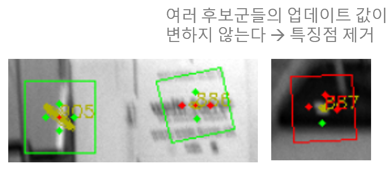
-
여러 점들 중 절반 이상 Innovation Term 값이 변하지 않는다면 해당 특징점을 제거한다
- 추가로 Heuristic Quality Score를 계산하여 점수가 Threshold보다 작으면 해당 특징점을 제거한다. Threshold 또한 전체 특징점 개수를 고려하여 Adaptive하게 변형한다.
- 1) Global Quality: 처음 탐지된 순간부터 얼마나 자주 트래킹 되는가
- 2) Local Quality: FOV 시야 안에 들어왔을 때 얼마나 자주 트래킹되는가
- 3) Local Visibility: FOV 시야 안에 얼마나 자주 보이는가
- 1) Global Quality: 처음 탐지된 순간부터 얼마나 자주 트래킹 되는가
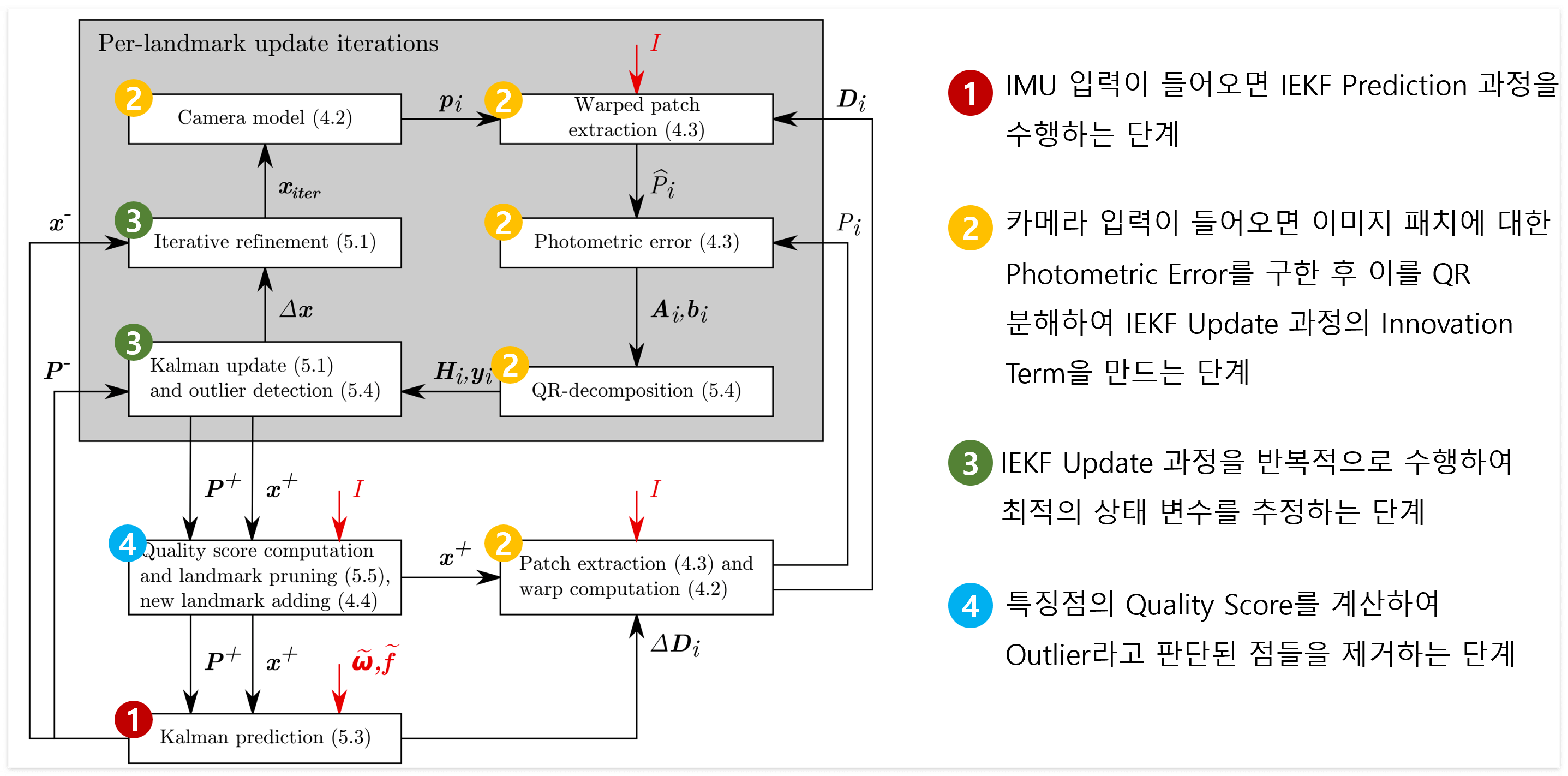
5. Overall flowchart
필자가 생각하는 ROVIO의 알고리즘 흐름도는 다음과 같다.
6. Derivation of state propagations
본 섹션에서는 ($\ref{eq:rovio1}$), ($\ref{eq:rovio2}$) 식에서 $\dot{\mathbf{r}}, \dot{\mathbf{v}}$와 $\dot{\mu}_{i}, \dot{\rho}_{i}$와 $\mu_{k+1}$ 수식의 유도 과정을 살펴본다. 해당 유도 과정는 ROVIO의 main contribution 중 하나로 [2]의 Appendix A 섹션에 자세히 설명되어 있다.
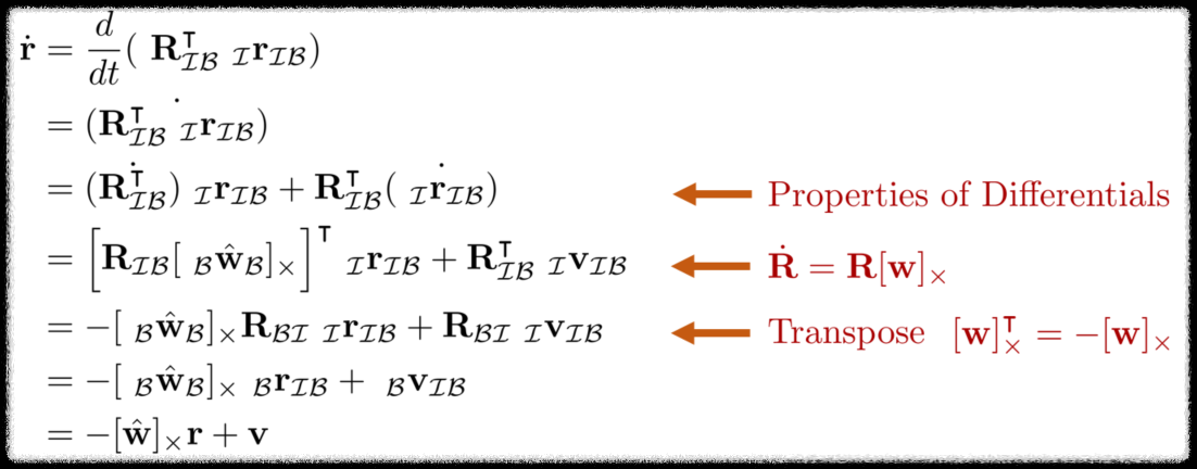
6.1. Derivation of $\dot{\mathbf{r}}, \dot{\mathbf{v}}$
($\ref{eq:rovio1}$)의 윗 두 줄을 보면 IMU의 위치와 속도에 대한 상태 방정식을 구하고 있다.
\begin{equation}
\begin{aligned}
& \dot{\mathbf{r}} = -[\hat{\mathbf{w}}]_{\times}\mathbf{r} + \mathbf{v} + w_{r} \\
& \dot{\mathbf{v}} = -[\hat{\mathbf{w}}]_{\times}\mathbf{v} + \hat{\mathbf{f}} + \mathbf{q}^{-1}(\mathbf{g}) \\
\end{aligned}
\end{equation}
- $\mathbf{r} = \ _{\mathcal{B}} \mathbf{r}_{\mathcal{I}\mathcal{B}}$ : robocentric 표현법을 통해 표현한 IMU 위치
- $\mathbf{v} = \ _{\mathcal{B}} \mathbf{v}_{\mathcal{B}}$ : robocentric 표현법을 통해 표현한 IMU 속도
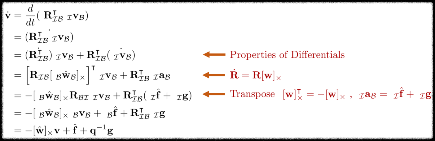
ROVIO에서는 회전에 대한 표현을 SO(3)군 $\mathbf{q} \in SO(3)$로 표현한다. $\mathbf{q}$는 회전 행렬이 될 수도 있고 쿼터니언이 될 수도 있는 순수한 회전에 대한 집합을 의미한다. 수식 유도에서는 이를 회전 행렬로 특정하여 사용한다. 즉, $\mathbf{q} \rightarrow \mathbf{R} \in \mathbb{R}^{3\times3}$을 사용한다. $\dot{\mathbf{r}}$를 자세히 풀어 쓰면 다음과 같다.
\begin{equation}
\begin{aligned}
\dot{\mathbf{r}}
& = \frac{d}{dt}( \ \mathbf{R}_{\mathcal{I}\mathcal{B}}^{\intercal} \ _{\mathcal{I}} \mathbf{r}_{\mathcal{I}\mathcal{B}} ) \\
& = \dot{ ( \mathbf{R}_{\mathcal{I}\mathcal{B}}^{\intercal} \ _{\mathcal{I}} \mathbf{r}_{\mathcal{I}\mathcal{B}} )} \\
& = \dot{ (\mathbf{R}_{\mathcal{I}\mathcal{B}}^{\intercal} ) } \ _{\mathcal{I}} \mathbf{r}_{\mathcal{I}\mathcal{B}} + \mathbf{R}_{\mathcal{I}\mathcal{B}}^{\intercal} \dot{ ( \ _{\mathcal{I}} \mathbf{r}_{\mathcal{I}\mathcal{B}} ) } \\
& = \Big[ \mathbf{R}_{\mathcal{I}\mathcal{B}} [ \ _{\mathcal{B}} \hat{\mathbf{w}}_{\mathcal{B}}]_{\times} \Big]^{\intercal} \ _{\mathcal{I}} \mathbf{r}_{\mathcal{I}\mathcal{B}}
+ \mathbf{R}_{\mathcal{I}\mathcal{B}}^{\intercal} \ _{\mathcal{I}} \mathbf{v}_{\mathcal{I}\mathcal{B}} \\
& = -[ \ _{\mathcal{B}} \hat{\mathbf{w}}_{\mathcal{B}}]_{\times} \mathbf{R}_{\mathcal{B}\mathcal{I}} \ _{\mathcal{I}} \mathbf{r}_{\mathcal{I}\mathcal{B}} + \mathbf{R}_{\mathcal{B}\mathcal{I}} \ _{\mathcal{I}} \mathbf{v}_{\mathcal{I}\mathcal{B}} \\
& = -[ \ _{\mathcal{B}} \hat{\mathbf{w}}_{\mathcal{B}}]_{\times} \ _{\mathcal{B}} \mathbf{r}_{\mathcal{I}\mathcal{B}} + \ _{\mathcal{B}} \mathbf{v}_{\mathcal{I}\mathcal{B}} \\
& = -[ \hat{\mathbf{w}}]_{\times} \mathbf{r} + \mathbf{v}
\end{aligned}
\end{equation}
다음으로 속도 $\dot{\mathbf{v}}$를 자세히 풀어 쓰면 다음과 같다.
\begin{equation}
\begin{aligned}
\dot{\mathbf{v}}
& = \frac{d}{dt}( \ \mathbf{R}_{\mathcal{I}\mathcal{B}}^{\intercal} \ _{\mathcal{I}} \mathbf{v}_{\mathcal{B}} ) \\
& = \dot{ ( \mathbf{R}_{\mathcal{I}\mathcal{B}}^{\intercal} \ _{\mathcal{I}} \mathbf{v}_{\mathcal{B}} )} \\
& = \dot{ (\mathbf{R}_{\mathcal{I}\mathcal{B}}^{\intercal} ) } \ _{\mathcal{I}} \mathbf{v}_{\mathcal{B}} + \mathbf{R}_{\mathcal{I}\mathcal{B}}^{\intercal} \dot{ ( \ _{\mathcal{I}} \mathbf{v}_{\mathcal{B}} ) } \\
& = \Big[ \mathbf{R}_{\mathcal{I}\mathcal{B}} [ \ _{\mathcal{B}} \hat{\mathbf{w}}_{\mathcal{B}}]_{\times} \Big]^{\intercal} \ _{\mathcal{I}} \mathbf{v}_{\mathcal{B}}
+ \mathbf{R}_{\mathcal{I}\mathcal{B}}^{\intercal} \ _{\mathcal{I}} \mathbf{a}_{\mathcal{B}} \\
& = -[ \ _{\mathcal{B}} \hat{\mathbf{w}}_{\mathcal{B}}]_{\times} \mathbf{R}_{\mathcal{B}\mathcal{I}} \ _{\mathcal{I}} \mathbf{v}_{\mathcal{B}} + \mathbf{R}_{\mathcal{I}\mathcal{B}}^{\intercal} ( \ _{\mathcal{I}} \hat{\mathbf{f}} + \ _\mathcal{I} \mathbf{g} ) \\
& = -[ \ _{\mathcal{B}} \hat{\mathbf{w}}_{\mathcal{B}}]_{\times} \ _{\mathcal{B}} \mathbf{v}_{\mathcal{B}} + \ _\mathcal{B} \hat{\mathbf{f}} + \mathbf{R}_{\mathcal{I}\mathcal{B}}^{\intercal} \ _\mathcal{I}\mathbf{g} \\
& = -[ \hat{\mathbf{w}}]_{\times} \mathbf{v} + \hat{\mathbf{f}} + \mathbf{q}^{-1} \mathbf{g}
\end{aligned}
\end{equation}
6.2. Derivation of $\dot{\mu}_{i}, \dot{\rho}_{i}$
먼저 $\dot{\mu}_{i}, \dot{\rho}_{i}$를 구하기 위해 다음 수식으로부터 시작한다.
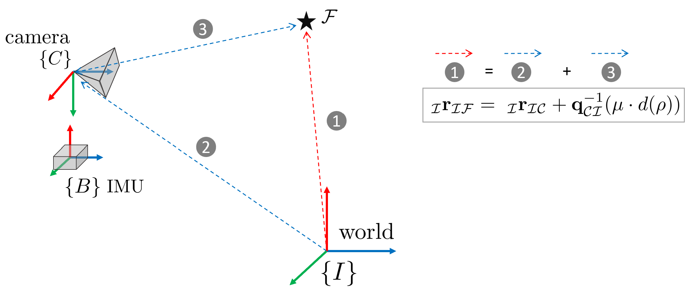
\begin{equation}
\begin{aligned}
\ _\mathcal{I}\mathbf{r}_{\mathcal{I}\mathcal{F}} = \ _\mathcal{I}\mathbf{r}_{\mathcal{I}\mathcal{C}} + \mathbf{q}_{\mathcal{C}\mathcal{I}}^{-1}(\mu \cdot d(\rho))
\end{aligned}
\end{equation}
- $\mathbf{q}_{\mathcal{C}\mathcal{I}}^{-1}$ : 카메라 좌표계 $\mathcal{C}$에서 본 벡터를 관성 좌표계 $\mathcal{I}$에서 본 벡터로 회전시켜주는 연산
- $\mu \cdot d(\rho)$ : 카메라 좌표계 $\mathcal{C}$에서 본 특징점의 3차원 위치
- $\mathbf{q}_{\mathcal{C}\mathcal{I}}^{-1}(\mu \cdot d(\rho)) = \ _\mathcal{I}\mathbf{r}_{\mathcal{C}\mathcal{F}}$와 같이 치환할 수 있다.
위 식은 그림에서 보는것과 같이 3차원 공간 상에 고정된 특징점(또는 랜드마크)가 주어졌을 때 이를 관성 좌표계 $\{\mathcal{I}\}$에서 바라본 벡터 $ _\mathcal{I}\mathbf{r}_{\mathcal{I}\mathcal{F}}$와 카메라를 경유하여 바라본 두 벡터들의 합 $ _\mathcal{I}\mathbf{r}_{\mathcal{I}\mathcal{C}} + \mathbf{q}_{\mathcal{C}\mathcal{I}}^{-1}(\mu \cdot d(\rho)$이 동일하다는 의미를 지닌다. 위 수식을 시간에 대해 미분한다.
\begin{equation} \label{eq:deriv1}
\begin{aligned}
\frac{d}{dt} \bigg\{ \ _\mathcal{I}\mathbf{r}_{\mathcal{I}\mathcal{F}} = \ _\mathcal{I}\mathbf{r}_{\mathcal{I}\mathcal{C}} + \mathbf{q}_{\mathcal{C}\mathcal{I}}^{-1}(\mu \cdot d(\rho)) \bigg\}
\end{aligned}
\end{equation}
좌측 항은 고정된 특징점이므로 $0$이 된다. 우측 첫번째 항은 $\frac{d}{dt}( \ _\mathcal{I}\mathbf{r}_{\mathcal{I}\mathcal{C}})=\ _\mathcal{I}\mathbf{v}_{\mathcal{I}\mathcal{C}}$와 같이 간단하게 변환되지만 우측 두번째 항은 아래와 같이 편미분을 수행해야 한다.
\begin{equation}
\begin{aligned}
\frac{d}{dt} \bigg\{ \mathbf{q}_{\mathcal{C}\mathcal{I}}^{-1}(\mu \cdot d(\rho)) \bigg\} = \frac{\partial \mathbf{A} } {\partial \mathbf{q}_{\mathcal{C}\mathcal{I}}} \dot{\mathbf{q}}_{\mathcal{C}\mathcal{I}} + \frac{\partial \mathbf{A} } {\partial \mu} \dot{\mu} + \frac{\partial \mathbf{A} } {\partial \rho} \dot{\rho}
\end{aligned}
\end{equation}
- $\mathbf{A} = \mathbf{q}_{\mathcal{C}\mathcal{I}}^{-1}(\mu \cdot d(\rho))$
- $\dot{\mathbf{q}}_{\mathcal{C}\mathcal{I}} = \frac{d}{dt}\mathbf{q}_{\mathcal{C}\mathcal{I}}$
- $\dot{\mu} = \frac{d}{dt}\mu$
- $\dot{\rho} = \frac{d}{dt}\rho$
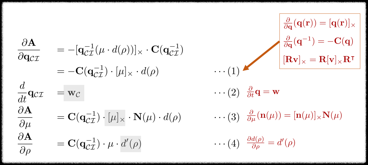
각각의 수식은 다음과 같이 유도할 수 있다.
\begin{equation}
\begin{aligned}
& \frac{\partial \mathbf{A} } {\partial \mathbf{q}_{\mathcal{C}\mathcal{I}}} &&= - [ \mathbf{q}_{\mathcal{C}\mathcal{I}}^{-1} ( \mu \cdot d(\rho))]_{\times} \cdot \mathbf{C}(\mathbf{q}^{-1}_{\mathcal{C}\mathcal{I}}) \\
& && = -\mathbf{C}(\mathbf{q}_{\mathcal{C}\mathcal{I}}^{-1}) \cdot [\mu]_{\times} \cdot d(\rho) &&& \quad \cdots \text{(1)} \\
& \frac {d } {dt} \mathbf{q}_{\mathcal{C}\mathcal{I}} && = \mathbf{w}_{\mathcal{C}} &&& \quad \cdots \text{(2)}\\
& \frac{\partial \mathbf{A} } {\partial \mu} && = \mathbf{C}(\mathbf{q}^{-1}_{\mathcal{C}\mathcal{I}}) \cdot [\mu]_{\times} \cdot \mathbf{N}(\mu) \cdot d(\rho) &&& \quad \cdots \text{(3)} \\
& \frac{\partial \mathbf{A} } {\partial \rho} && = \mathbf{C}(\mathbf{q}^{-1}_{\mathcal{C}\mathcal{I}}) \cdot \mu \cdot d'(\rho) &&& \quad \cdots \text{(4)}
\end{aligned}
\end{equation}
지금까지 유도한 수식을 모두 통합하여 ($\ref{eq:deriv1}$)을 다시 작성하면 다음과 같다.
\begin{equation}
\begin{aligned}
0 = & \ _\mathcal{I}\mathbf{v}_{\mathcal{I}\mathcal{C}} -\mathbf{C}(\mathbf{q}_{\mathcal{C}\mathcal{I}}^{-1}) \cdot [\mu]_{\times} \cdot \mathbf{w}_{\mathcal{C}} \cdot d(\rho) \\
& + \mathbf{C}(\mathbf{q}^{-1}_{\mathcal{C}\mathcal{I}}) \bigg( [\mu]_{\times} \cdot \mathbf{N}(\mu) \cdot d(\rho) \cdot \dot{\mu} + \mu \cdot d'(\rho) \cdot \dot{\rho} \bigg)
\end{aligned}
\end{equation}
위 식의 양 변의 왼쪽에 $\mathbf{C}(\mathbf{q}_{\mathcal{C}\mathcal{I}})$를 곱하면 다음과 같다.
\begin{equation}
\begin{aligned}
0 = & \mathbf{v}_{\mathcal{I}\mathcal{C}} - [\mu]_{\times} \cdot \mathbf{w}_{\mathcal{C}} \cdot d(\rho) \\
& + [\mu]_{\times} \cdot \mathbf{N}(\mu) \cdot d(\rho) \cdot \dot{\mu} + \mu \cdot d'(\rho) \cdot \dot{\rho}
\end{aligned}
\end{equation}
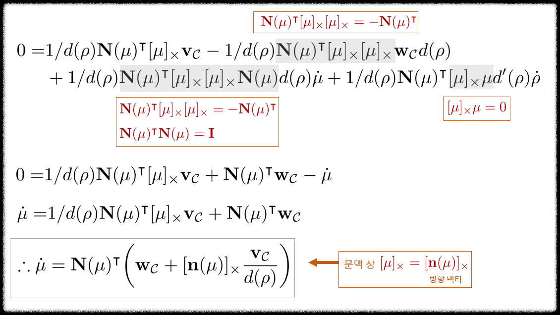
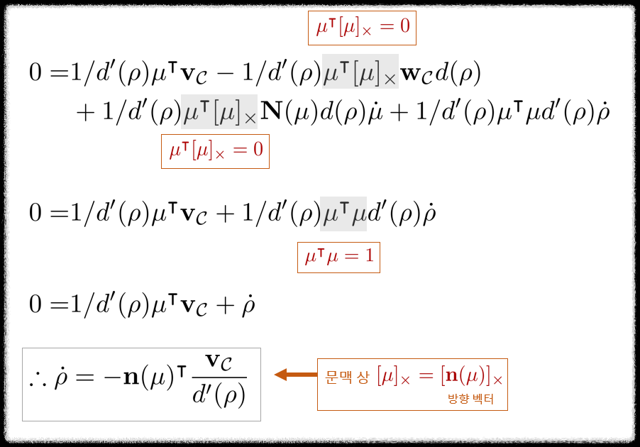
$\dot{\mu}$를 구하기 위해 위 식의 양변에 $1/d(\rho)\mathbf{N}(\mu)^{\intercal}[\mu]_{\times}$를 곱한 후 정리하고, $\dot{\rho}$를 구하기 위해 위 식의 양변에 $1/d'(\rho)\mu^{\intercal}$을 곱한 후 정리하면 ($\ref{eq:rovio1}$) 아래 두 줄과 같은 식을 얻을 수 있다.
\begin{equation}
\boxed{ \begin{aligned}
& \dot{\mu} = \mathbf{N}(\mu)^{\intercal} \bigg( \mathbf{w}_{\mathcal{C}} + [\mathbf{n}(\mu)]_{\times} \frac{\mathbf{v}_{\mathcal{C}}}{d(\rho)} \bigg) \\
& \dot{\rho} = -\mathbf{n}(\mu)^{\intercal} \frac{\mathbf{v}_{\mathcal{C}}}{d'(\rho)}
\end{aligned} }
\end{equation}
자세한 유도 과정의 그림을 아래 첨부하였다.
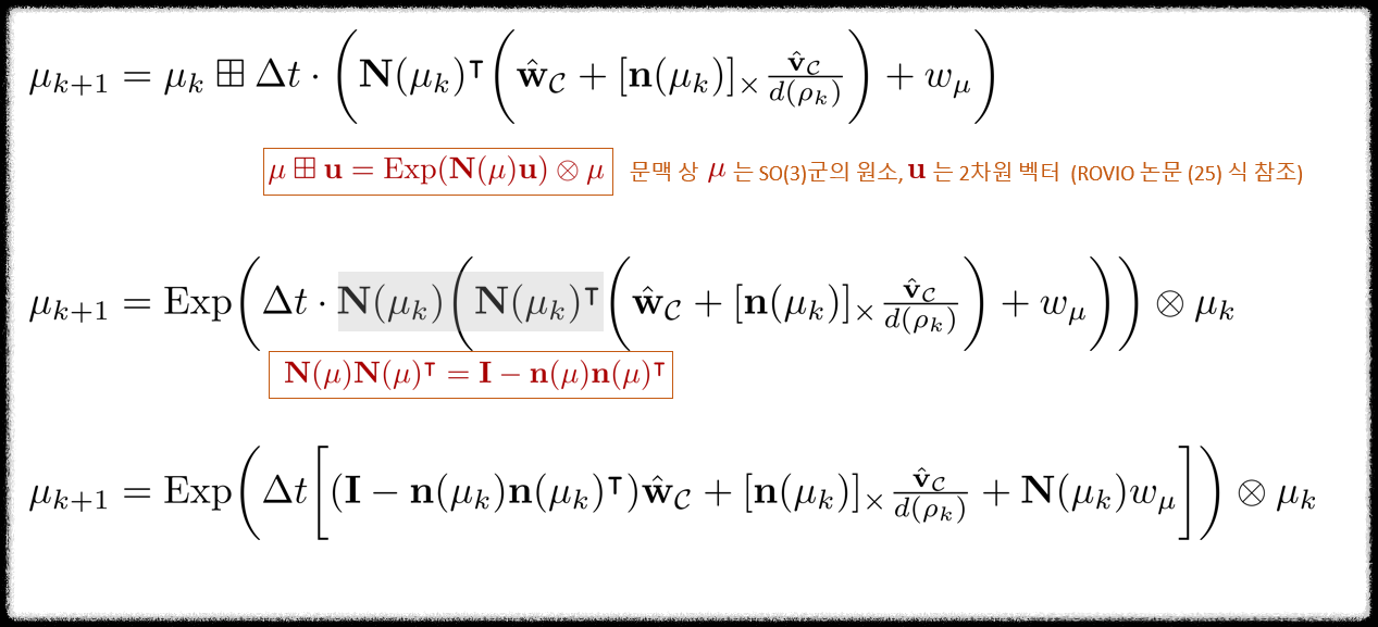
6.3. Derivation of discrete $\mu_{k+1}$
본 섹션에서는 ($\ref{eq:rovio2}$)에서 $\mu_{k+1}$ 식을 유도하는 과정에 대해 설명한다. State propagation 공식에 의해 $\mu_{i,k+1}$는 다음과 같은 수식이 된다.
\begin{equation}
\begin{aligned}
\mu_{k+1} = \text{Exp} \bigg( \Delta t \bigg[ (\mathbf{I} - \mathbf{n}(\mu_{k})\mathbf{n}(\mu_{k})^{\intercal} )\hat{\mathbf{w}}_{\mathcal{C}} + [\mathbf{n}(\mu_{k})]_{\times} \frac{\hat{\mathbf{v}}_{\mathcal{C}}}{d(\rho_{k})} + \mathbf{N}(\mu_{k})w_{\mu} \bigg] \bigg) \otimes \mu_{k}
\end{aligned}
\end{equation}
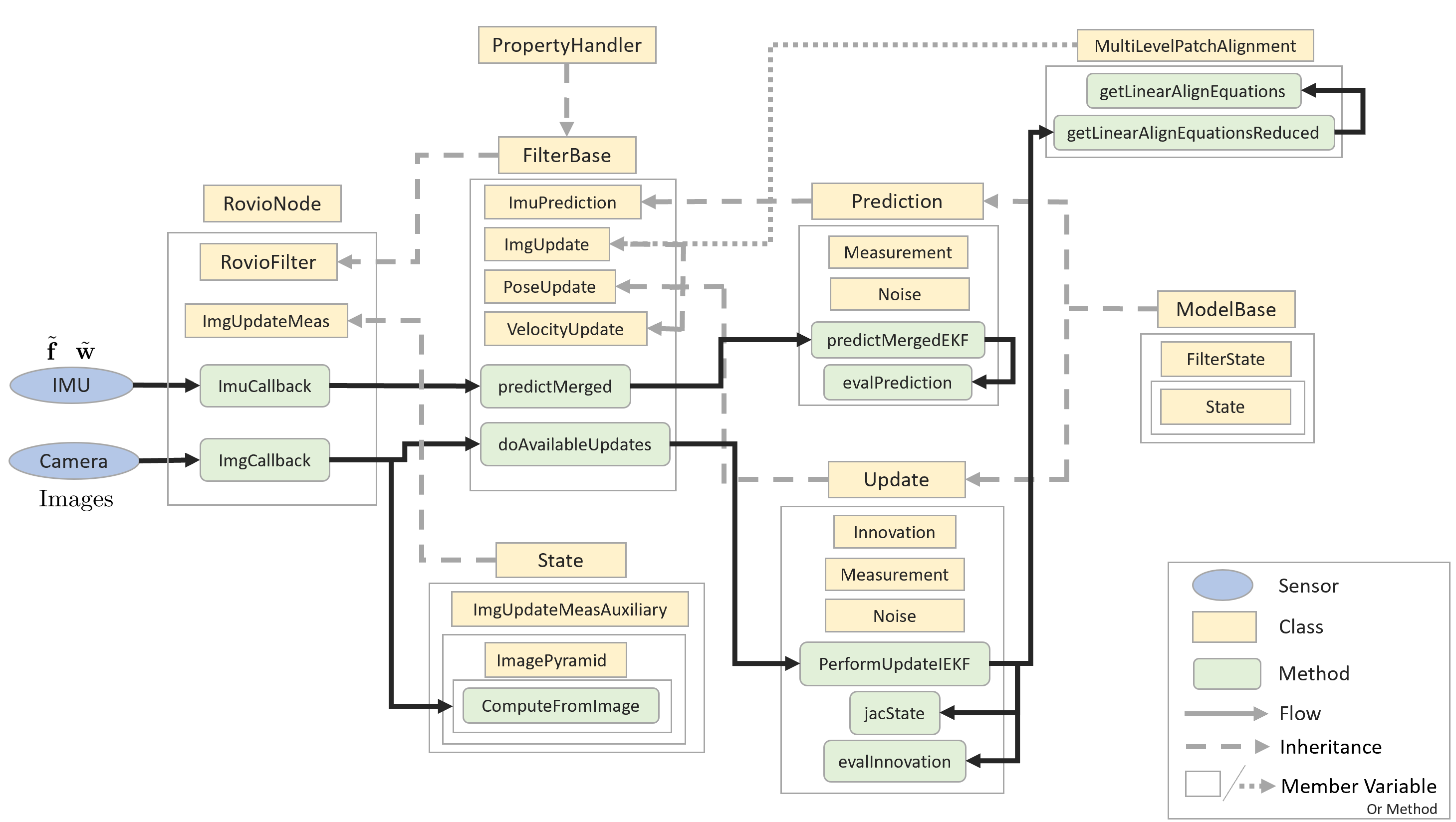
7. Code review
ROVIO 코드의 클래스 간 상관 관계는 다음과 같이 구성되어 있다.
8. References
[3] ROVIO analysis document by Steven Cui
[4] A Quick Guide for the Iterated Extended Kalman Filter on Manifolds by Jianzhu Huai, Xiang Gao
[5] A Primer on the Differential Calculus of 3D Orientations, M. Bloesch et al., 2016, arXiv
'Engineering' 카테고리의 다른 글
| [SLAM] FAST-LIO2 논문 리뷰 (+ IKF, ikd-tree) (30) | 2024.04.17 |
|---|---|
| [SLAM] VINS-mono 논문 리뷰 (+ IMU preintegration) (11) | 2022.10.15 |
| [MVG] Stereo Camera Calibration 예제코드 및 설명 (C++) (3) | 2022.07.14 |
| [MVG] Scene Plane-based Homography 예제코드 및 설명 (C++) (0) | 2022.07.07 |
| [MVG] Vanishing Point-based Metric Rectification 예제코드 및 설명 (C++) (0) | 2022.07.03 |


