 A L I D A
In this post, Lie Theory used in SLAM is explained. When studying the optimization part in SLAM, Lie Theory-based optimization methods often appear, but it is difficult to understand the optimization process without prior knowledge of the content. did Most of the contents were referred to [6].
Group Theory
A group refers to an algebraic structure consisting of a set and a binary operation, which is an operation of two elements. For example, when a set is called $A$ and a certain binary operation is expressed as $*$, the group can be expressed as $G = (A, *)$. A set of generally known numbers such as integers, rational numbers, real numbers, and complex numbers, and operations such as addition and multiplication, belong to the group.
Groups generally have the following characteristics.
- Associativity: The associative law of $(a* b) * c = a * (b * c)$ is established for any three elements $a,b,c \in G$ in the group.
- Identity element: For any element $a \in G$ in a group, $e \in G$ that satisfies $a * e = a = e * a$ exists, then $e$ is said to be an identity element.
- Inverse: For any element $a \in G$ in the group, if there exists an element $x \in G$ that satisfies $a* x = e = x * a$, $x$ is said to be an inverse. The inverse is also expressed as $a^{-1}$
- Composition: $a*b \in G$ holds for any two elements $a,b \in G$ in the group. At this time, for most groups, the binary operation $*$ is not commutative. That is, $a*b \neq b*a$.
Lie Group
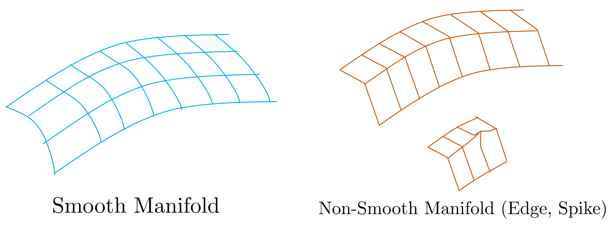
Among several groups, the Lie Group means a group having a smooth manifold. At this time, the smooth manifold means a manifold in a smooth state where all elements of the group do not have edges and spikes as shown in the figure above, and the lie group means a group in which all elements exist on this smooth manifold. All elements on the smooth manifold are characterized by being differentiable.
Manifold
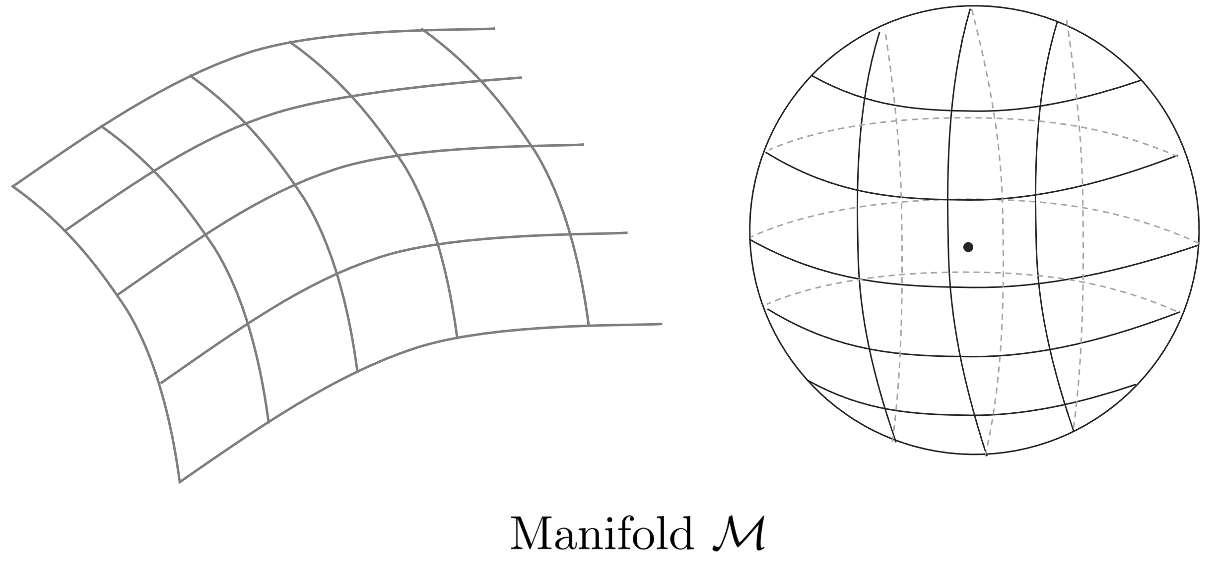
An N-dimensional manifold $\mathcal{M}$ is a geometric space with Euclidean structure locally for any point $\mathbf{x}\in\mathcal{M}$ inside $\mathcal{M}$. it means. In other words, all points that exist near $\mathbf{x}$ are homeomorphic in $\mathbb{R}^{N}$ space. Intuitively, manifold means the constraint space of the group.
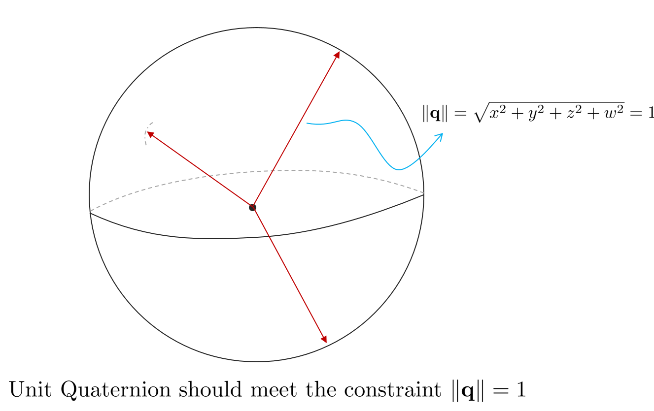
For example, in order for any quaternion $\mathbf{q}=[x,y,z,w]$ to be used as a 3-dimensional rotation operator, it must satisfy the property of a unit quaternion, and the constraint at this time is $\| \mathbf{q} \| = 1$. That is, $\mathbf{q}$ must satisfy a point on the surface of a 4-dimensional sphere, and this 4-dimensional sphere is called a unit quaternion manifold. Constraints of more than 4 dimensions cannot be visualized on a plane, so they are generally explained using a 3-dimensional sphere.
In the case of SE(3) Lie Group, which will be described later, a 6-dimensional element must satisfy certain constraints. That is, the elements of the SE(3) Lie Group must exist on the 6-dimensional manifold. Since this cannot be explained on a plane, it is explained using a three-dimensional sphere.
Group Action
One of the characteristics of a group is that it can transform (=act) another set or group. This means that a group can act as an operator to transform a particular set. This means that Lie Theory is an appropriate tool for expressing the movement of objects in 3D space.
Given $a,b \in G$ and $v \in V$, and the binary operation $*$, the conversion rule satisfies
- Applying the identity element $e$ causes no conversion. $e * v = v$
- The associative law applies to both conversion operations. $(a*b)*v = a*(b*v)$
Topology of Lie Theory
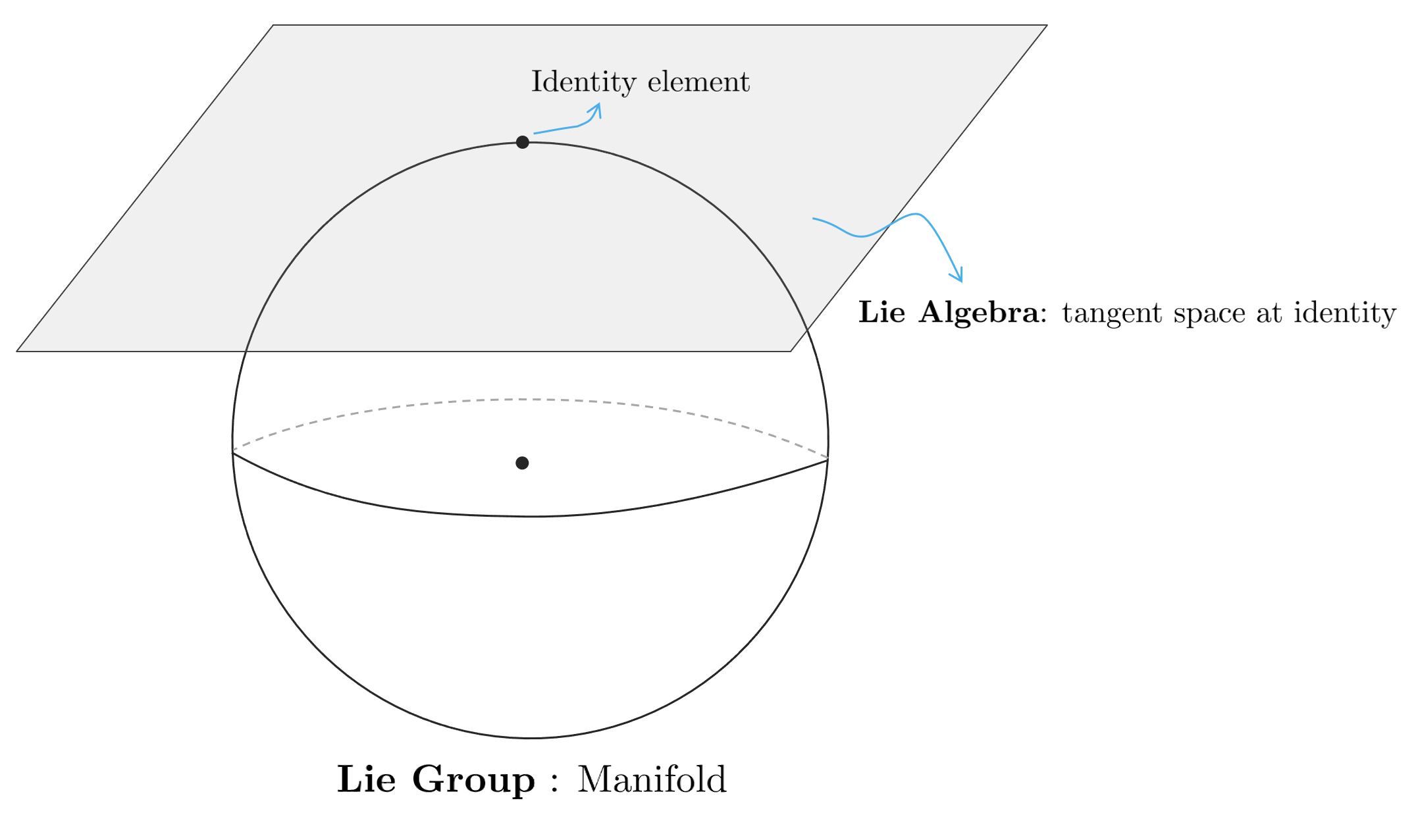
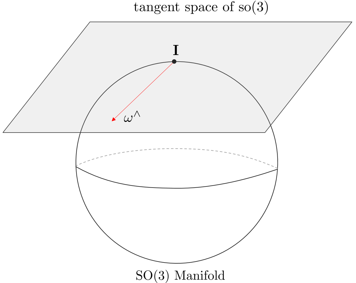
The geometric structure of Lie Theory is shown in the figure above.
- A Lie Group means a set of points on one manifold with constraints and has a non-linear property.
- Lie Algebra means the tangent space at the identity element, which is a point on the manifold. At this time, the tangent plane of Lie Algebra is valid only when it is in contact with the identity element and has the characteristic of a linear vector space.
The reason Lie Group and Lie Algebra are important is that 1:1 conversion is possible between the two spaces. Therefore, instead of directly operating in a non-linear manifold space (Lie Group) with complex constraints, a method of performing an operation in a relatively simple linear vector space (Lie Algebra) and then converting it to a manifold space is used. The operations that make this possible are Exponential Mapping and Logarithm Mapping.
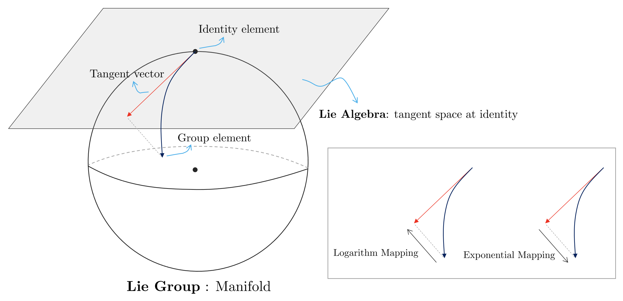
Exponential Mapping means the operation of converting Lie Algebra → Lie Group, and Logarithm Mapping means the opposite operation of converting Lie Group → Lie Algebra.
Plus and Minus Operators of Lie Group
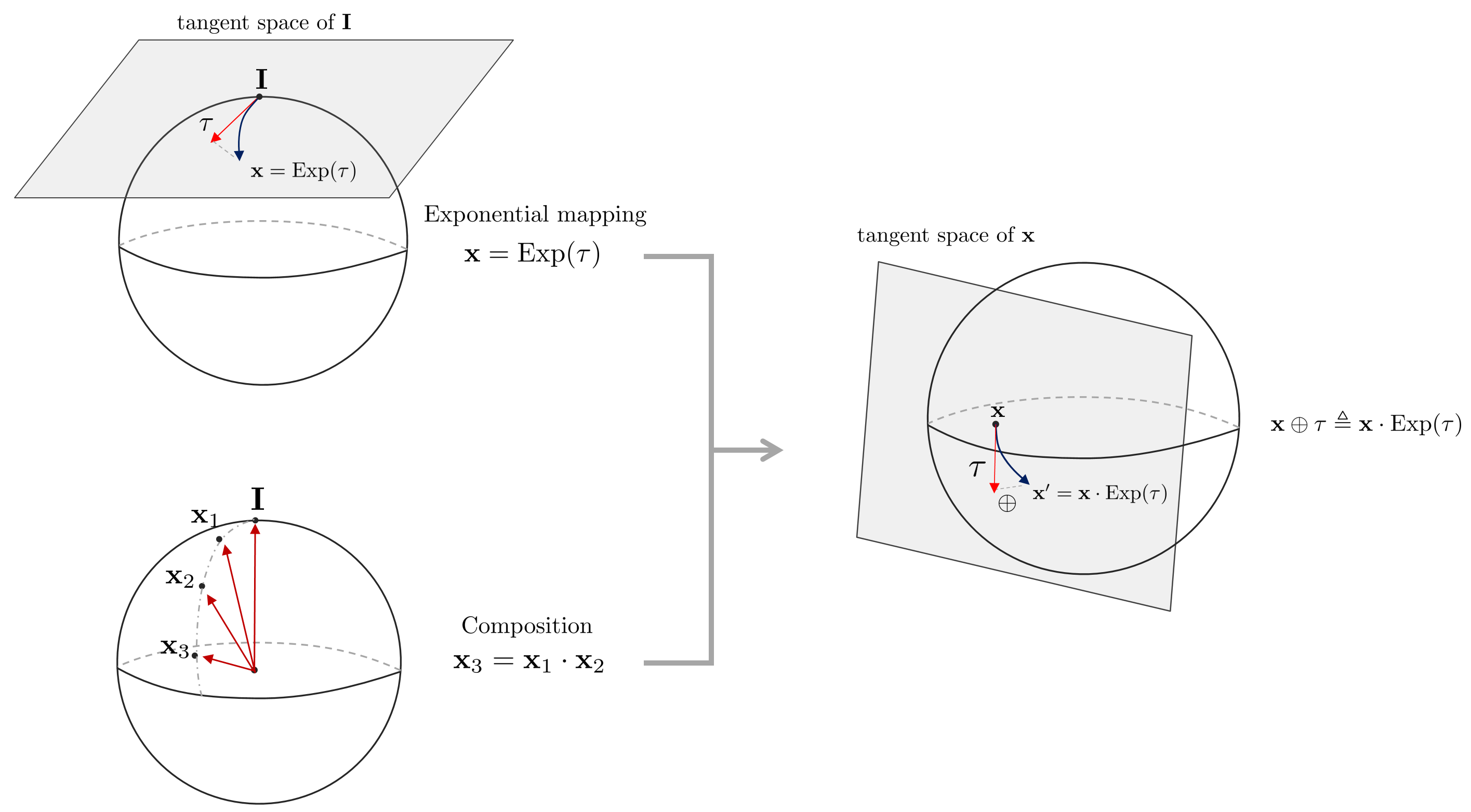
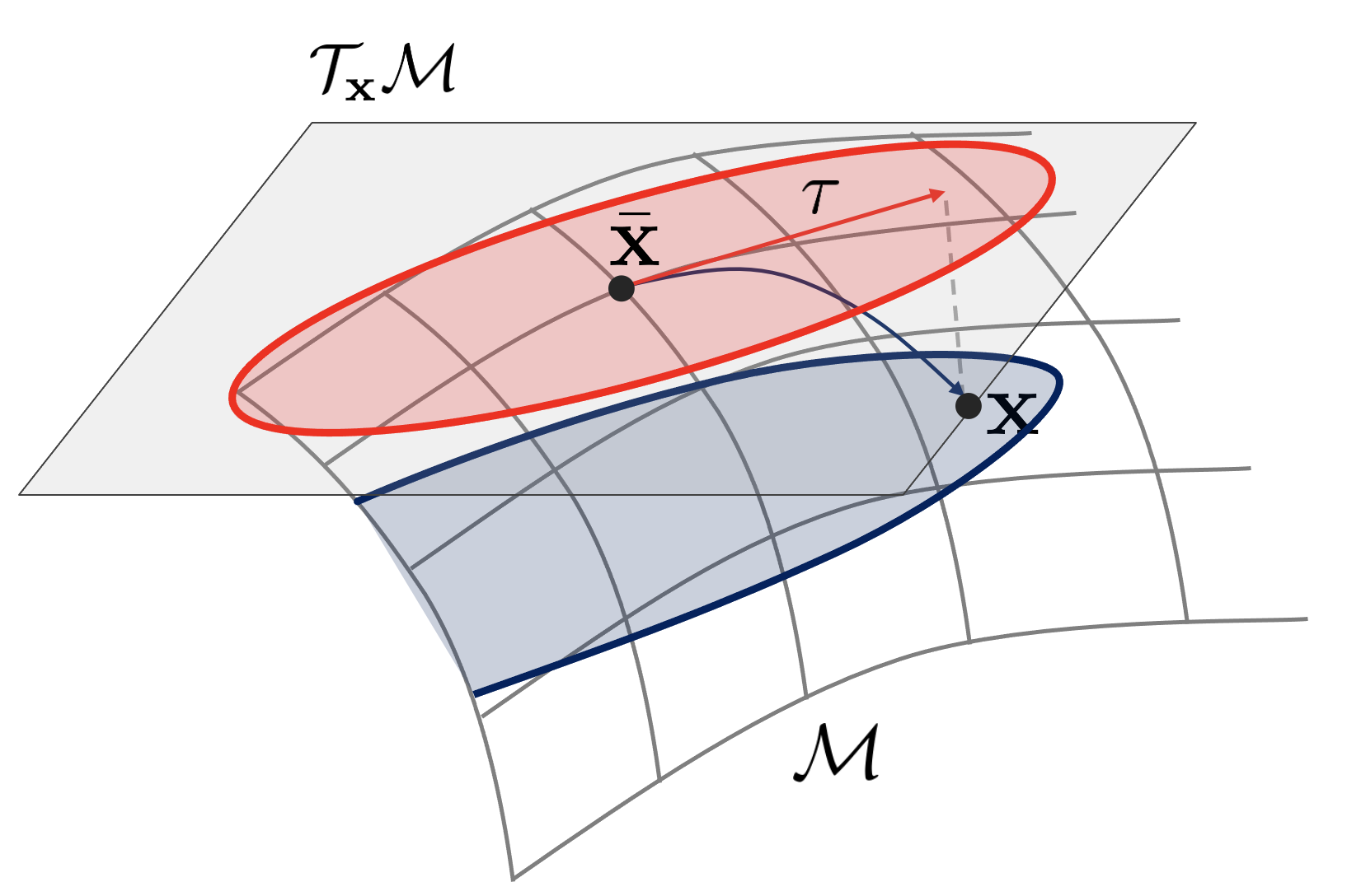
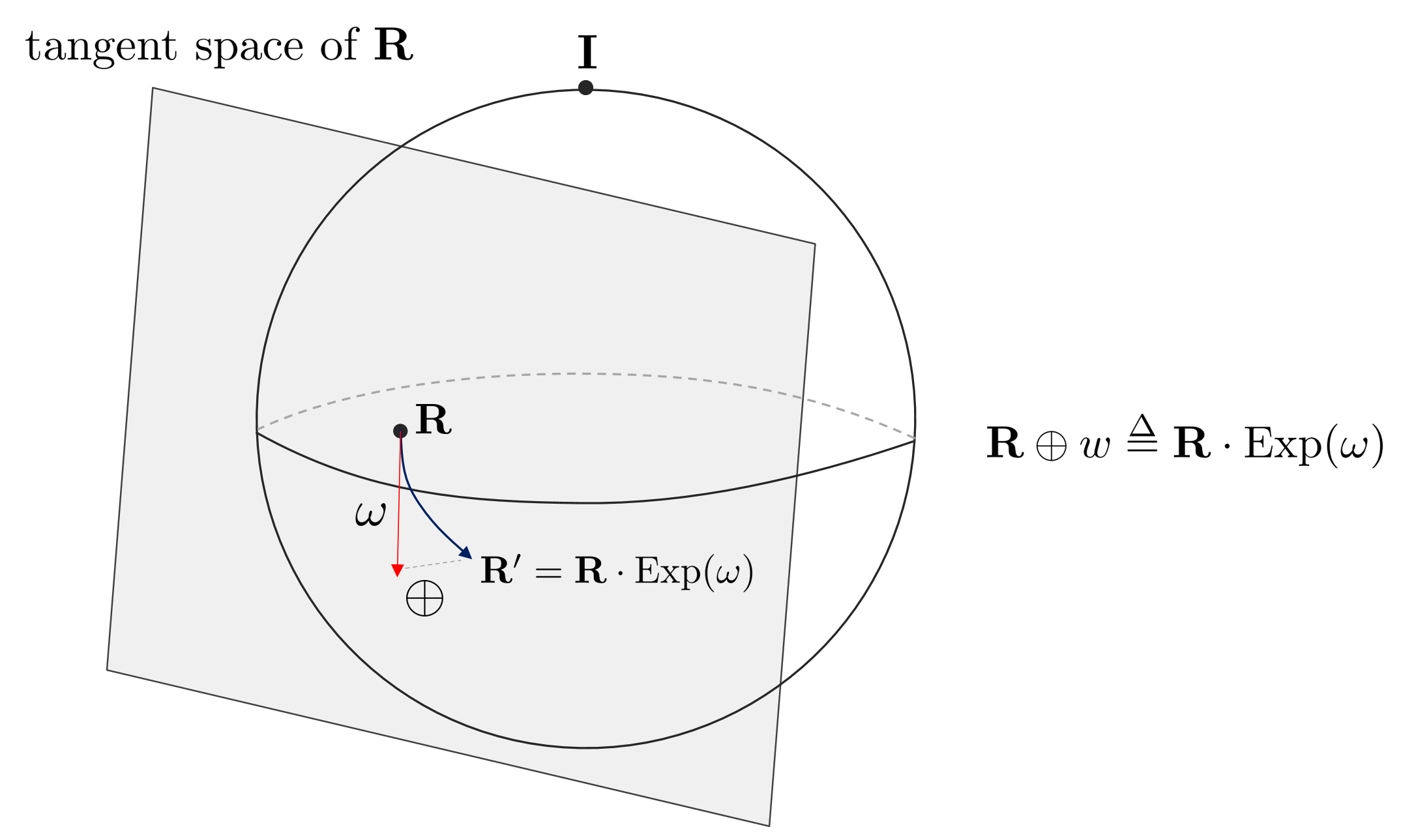
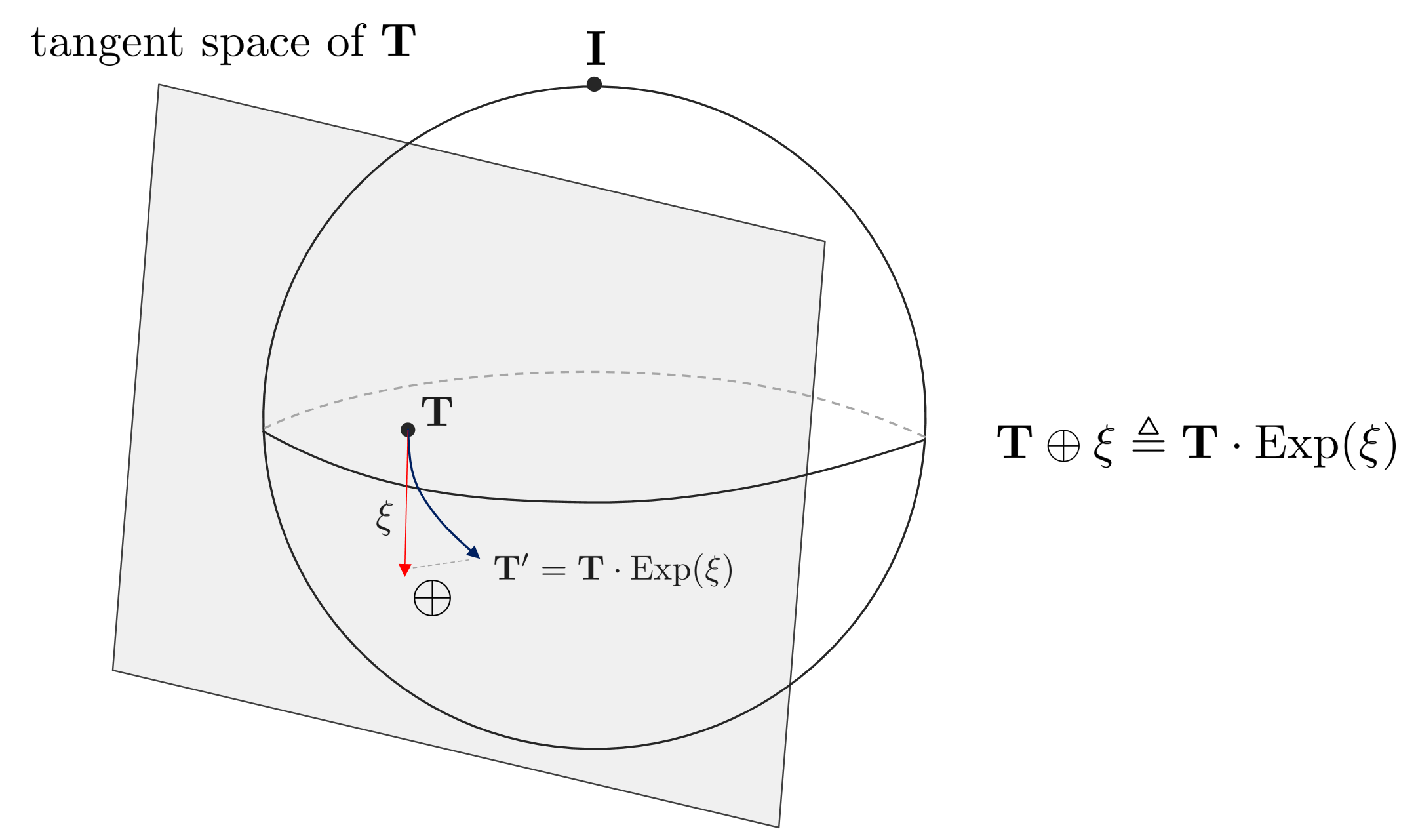
Using the exponential mapping described above, the element $\mathbf{x}$ of the Lie Group can be transformed using an arbitrary Lie Algebra $\tau$. At this time, since general $+,-$ operators are not applied between Lie Group elements, new $\oplus, \ominus$ operators must be defined. First of all, the $\oplus$ operator is an operator that applies an additional conversion as much as $\tau$ to an arbitrary Lie Group element $\mathbf{x}$.
$$\mathbf{x} \oplus \tau \triangleq \mathbf{x} \cdot \text{Exp}(\tau)$$
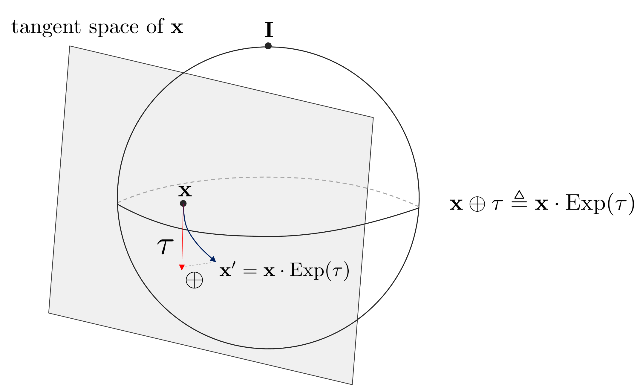
At this time, the $\tau$ vector on the $\mathbf{x}$ tangent plane is treated as the same as the $\tau$ vector on the identity element tangent plane due to the lie group composition property.
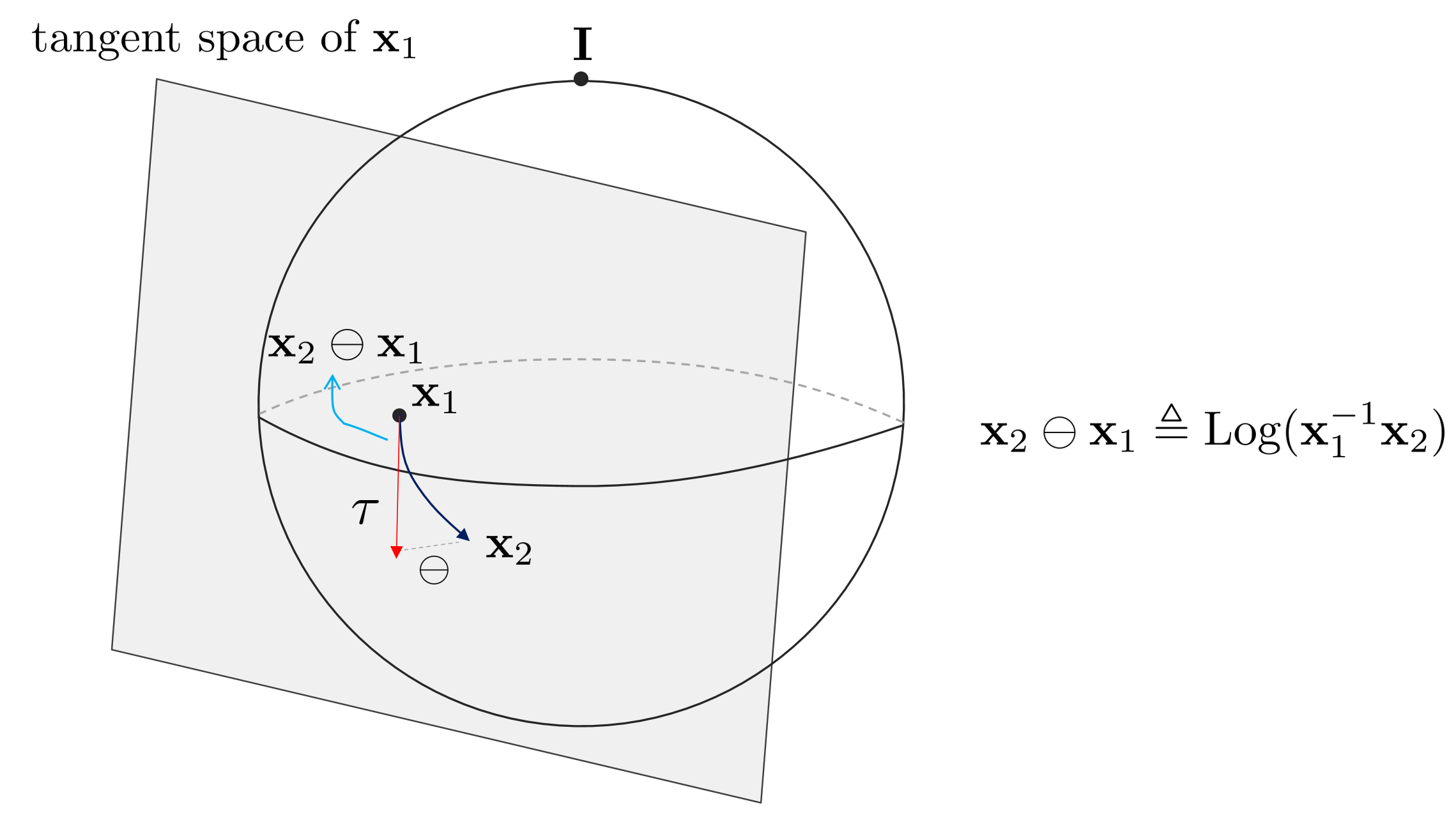
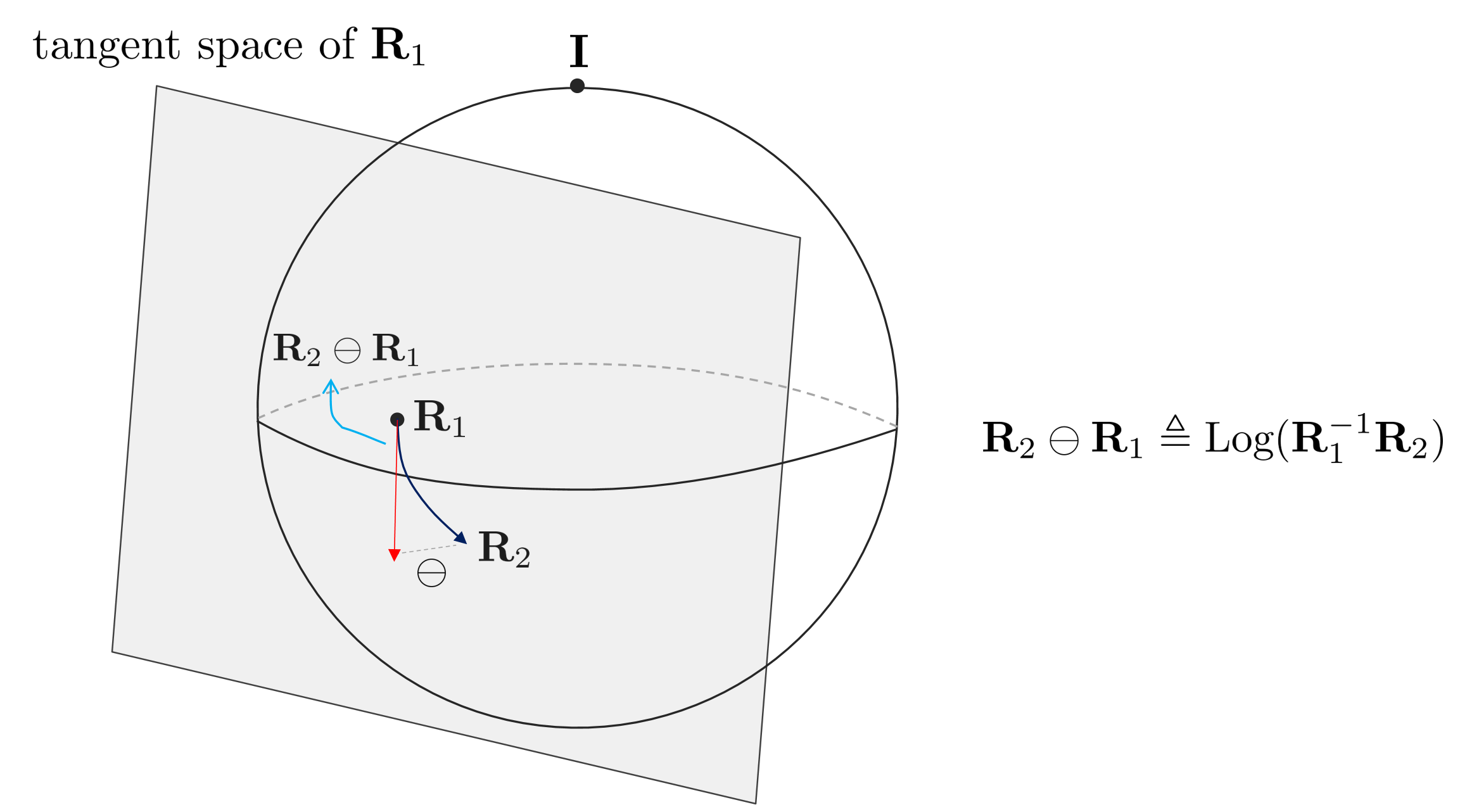
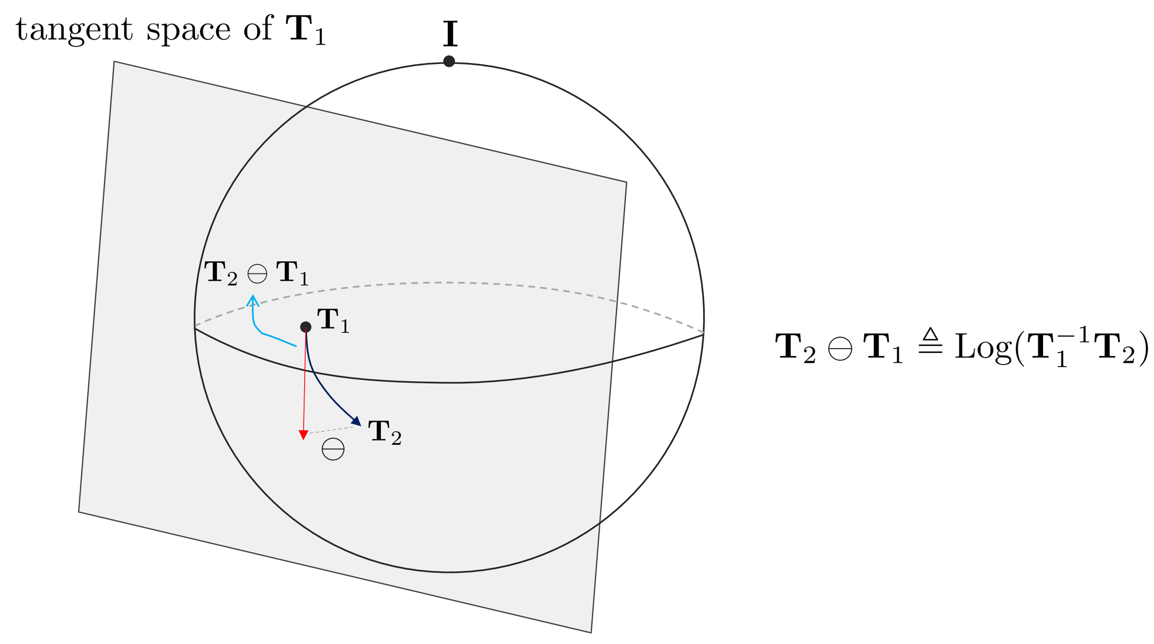
Conversely, the $\ominus$ operator is used with $\mathbf{x}_{2} \ominus \mathbf{x}_{1}$ when there are two Lie Group elements $\mathbf{x}_{1}, \mathbf{x}_{2}$, and means the relative change of $\mathbf{x}_{2}$ from $\mathbf{x}_{1}$.
$$\mathbf{x}_{2} \ominus \mathbf{x}_{1} \triangleq \text{Log}(\mathbf{x}_{1}^{-1}\mathbf{x}_{2})$$
Tangent Space and Lie Algebra
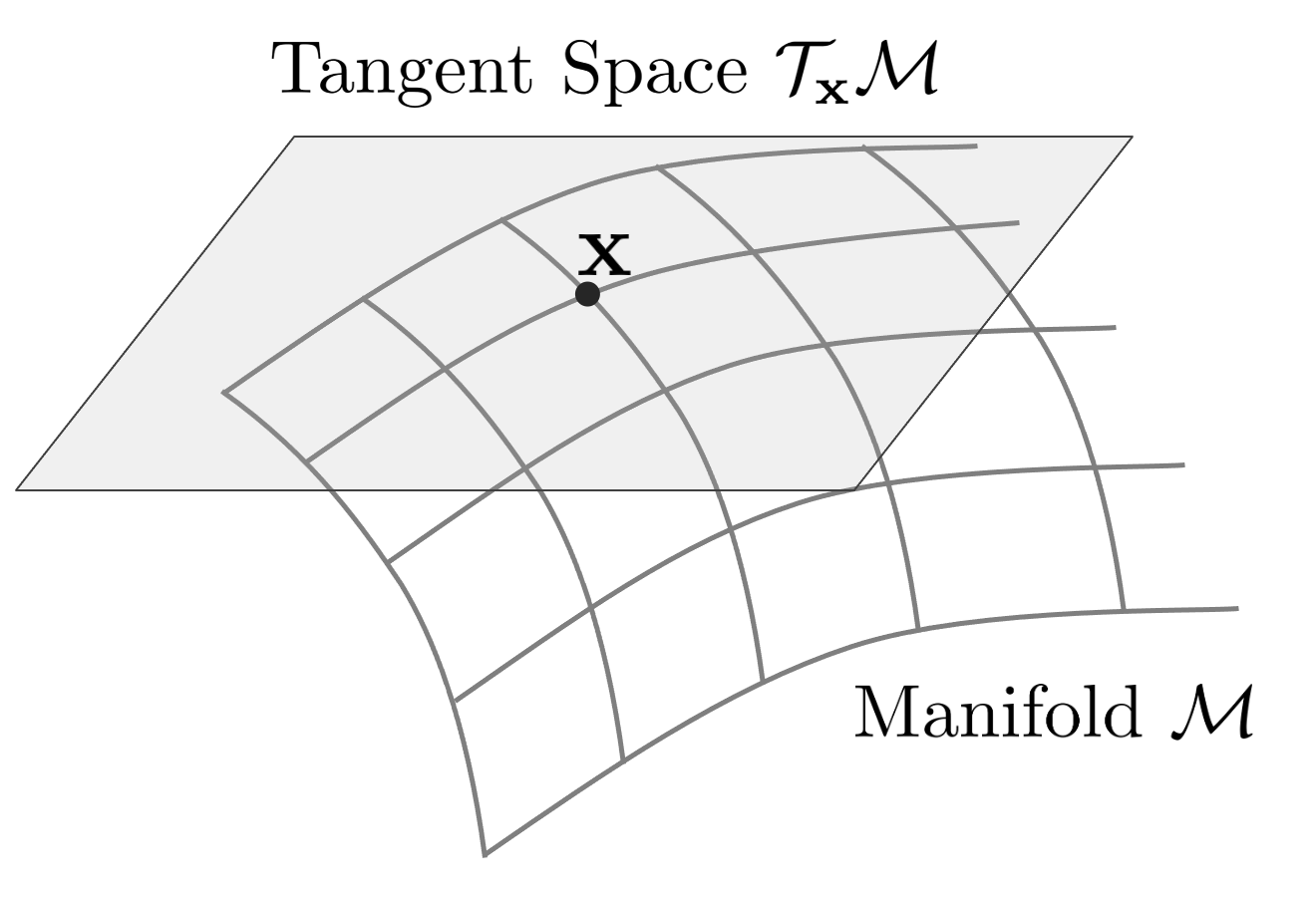
When a point $\mathbf{x} \in \mathcal{M}$ exists on any manifold $\mathcal{M}$, the tangent plane to it is represented as $\mathcal{T}_{\mathbf{x}}\mathcal{M}$.
- The tangent plane $\mathcal{T}_{\mathbf{x}}\mathcal{M}$ is uniquely determined for an arbitrary point, and since it is a vector space, calculus can be performed.
- The dimension of the tangent plane is determined by the number of degrees of freedom of the manifold. That is, since SO(3) has 3 degrees of freedom for rotation, so(3) has a 3-dimensional tangent plane, and since SE(3) has 6 degrees of freedom for pose, se(3) has a 6-dimensional tangent plane.
- The tangent plane in the identity element is specifically called Lie Algebra.
Calculus on Lie Group
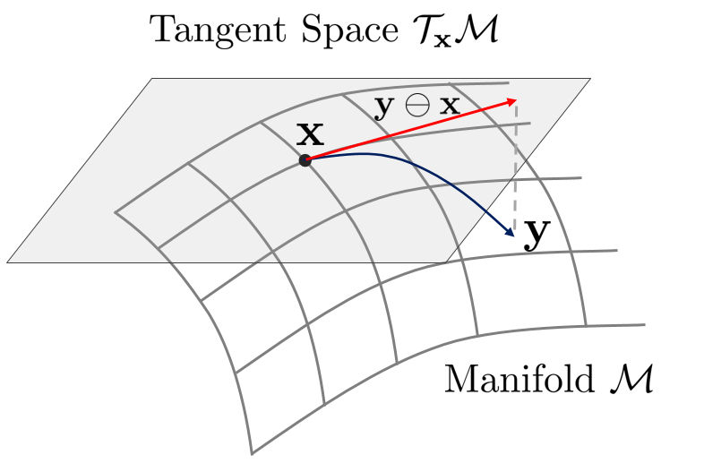
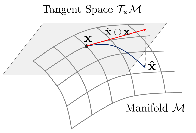
Suppose there are two elements $\mathbf{x}$ and $\mathbf{y}$ on the Lie Group. At this time, the difference between the two elements can be expressed on the tangent plane as $\mathbf{y} \ominus \mathbf{x}$ using the $\ominus$ operator. As described above, since the tangent plane $\mathcal{T}_{\mathbf{x}}\mathcal{M}$ is a linear vector space, it is relatively easy to calculate jacobian and covariance. This characteristic is a key reason why Lie Theory can be used for optimization calculations. For example, when two elements are relatively close, it can be used for error function modeling.
$$\mathbf{e} = \hat{\mathbf{x}} \ominus \mathbf{x}$$
Jacobians on Lie Group
Suppose we are given a vector function $f(\mathbf{x})$ that exists in a linear vector space. At this time, $f(\mathbf{x})$ is a function that satisfies $\mathbf{x} \in \mathbb{R}^{n}, f(\mathbf{x}) \in \mathbb{R}^{m}$.
$$f : \mathbb{R}^{n} \mapsto \mathbb{R}^{m}$$
At this time, the first partial derivative of the vector function becomes a matrix, which is specifically called Jacobian.
$$\mathbf{J} = \begin{bmatrix} \frac{\partial f_{1}}{\partial x_{1}} & \cdots & \frac{\partial f_{1}}{\partial x_{n}} \\ \vdots & \ddots & \vdots \\ \frac{\partial f_{m}}{\partial x_{1}} & \cdots & \frac{\partial f_{m}}{\partial x_{n}} \end{bmatrix}$$
If this is expressed using the small amount of change $\mathbf{h}$, it is as follows.
$$\mathbf{J} = \frac{\partial f(\mathbf{x})}{\partial \mathbf{x}} \triangleq \lim_{\mathbf{h \rightarrow 0}} \frac{f(\mathbf{x} + \mathbf{h}) - f(\mathbf{x}) }{\mathbf{h}} \in \mathbb{R}^{m \times n}$$
As above, in a linear vector space, the Jacobian can be calculated using the $+$ and $-$ operators. However, in the case of elements of Lie Group, the Jacobian cannot be expressed through the existing method because the group is not closed by $+ and -$ operations as described above.
Suppose that the vector function $f(\mathbf{x})$ existing on the Lie Group is given as follows.
$$f : \mathcal{M} \mapsto \mathcal{N} ; \mathbf{x} \mapsto \mathbf{y} = f(\mathbf{x})$$
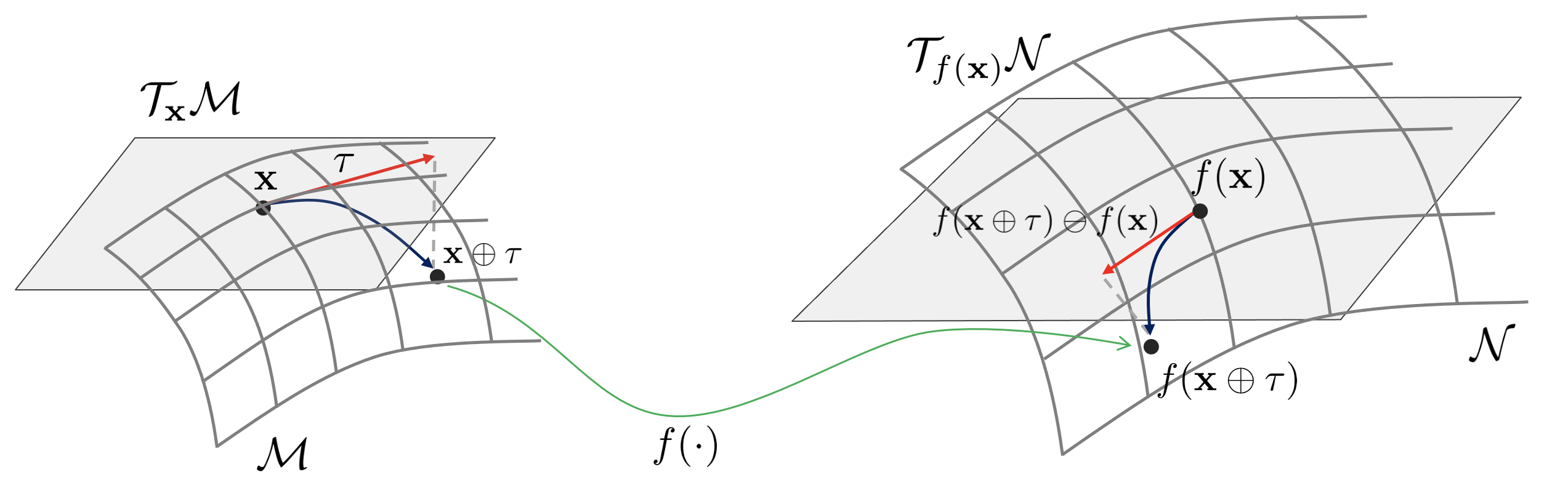
This means that function $f$ maps element $\mathbf{x}$ on manifold $\mathcal{M}$ to element $\mathbf{y}$ on another manifold $\mathcal{N}$. say function The Jacobian for this can be expressed as:
$$\mathbf{J} = \frac{D f(\mathbf{x})}{D \mathbf{x}} = \lim_{\tau \rightarrow 0} \frac{f(\mathbf{x} \oplus \tau) \ominus f(\mathbf{x})}{\tau} \in \mathbb{R}^{m \times n}$$
The Jacobian $\mathbf{J}$ converts the elements above $\mathcal{T}_{\mathbf{x}}\mathcal{M}$ to $\mathcal{T}_{f(\mathbf{x}) } \mathcal{N}$ can be thought of as a function that maps to the element above. If this is shown in a picture, it is as follows.
Perturbations on Lie Group
Using the property that the tangent plane is a linear vector space, Lie Group elements can be modeled as perturbation of random variables.
$$\mathbf{x} = \bar{\mathbf{x}} \oplus \tau \quad \text{where, } \tau = \mathbf{x}\ominus \bar{\mathbf{x}}$$
$$\mathbf{P}_{\mathbf{x}} = \mathbb{E}[\tau \cdot \tau^{\intercal}]$$
$$\mathbf{P}_{\mathbf{x}} = \mathbb{E}[(\mathbf{x}\ominus\bar{\mathbf{x}})\cdot(\mathbf{x}\ominus\bar{\mathbf{x}})^{\intercal}]$$
If given a function $\mathbf{y} = f(\mathbf{x})$, the Jacobian is $\mathbf{J} = \frac{D\mathbf{y}}{D\mathbf{x }}$, and through this, the covariance $\mathbf{P}_{\mathbf{y}}$ can be obtained as follows.
$$\mathbf{P}_{\mathbf{y}} = \mathbf{J} \cdot \mathbf{P}_{\mathbf{x}} \cdot \mathbf{J}^{\intercal}$$
This is equivalent to the propagataion formula for covariance in vector space.
SO(3) Group
Lie Group SO(3)
The Special Orthogonal 3 (SO(3)) group, one of the Lie groups, means a group consisting of a 3D Rotation Matrix and operations closed to it, and is used to express the rotation of a 3D object.
\begin{equation}\begin{aligned}
SO(3) = \{ \mathbf{R} \in \mathbb{R}^{3 \times 3} \ | \ \mathbf{R}\mathbf{R}^{T} = \mathbf{I}, \text{det}(\mathbf{R})=1 \}
\end{aligned}
\end{equation}
The composition operation and inverse operation of the SO(3) group are expressed through matrix multiplication and inverse matrix.
Lie Algebra so(3)
Lie Algebra so(3) of the SO(3) family is an skew-symmetric matrix of the size of $\mathbb{R}^{3\times 3}$ as follows.
\begin{equation}
\begin{aligned}
\text{so}(3) = \{ \ \omega^{\wedge} = \begin{bmatrix} 0&-\omega_{z}&\omega_{y} \\ \omega_{z}&0&-\omega_{x} \\ -\omega_{y}&\omega_{x}&0 \end{bmatrix} \in \mathbb{R}^{3\times 3} \ | \ \omega = \begin{bmatrix} w_{x}\\w_{y}\\w_{z} \end{bmatrix}\in \mathbb{R}^{3} \ \}
\end{aligned}
\end{equation}
The generators in so(3) are derived from rotation about each axis at the origin. Generators mean basis matrices that are orthogonal to each other.
\begin{equation}
\begin{aligned}
& G_{1} = \begin{pmatrix} 0&0&0 \\ 0&0&-1 \\ 0&1&0 \end{pmatrix}, \ \ G_{2} = \begin{pmatrix} 0&0&1 \\ 0&0&0 \\ -1&0&0 \end{pmatrix},\ \ G_{3} = \begin{pmatrix} 0&-1&0 \\ 1&0&0 \\ 0&0&0 \end{pmatrix} \\
\end{aligned}
\end{equation}
Each element of so(3) can be expressed as a linear combination of constructors.
\begin{equation}
\begin{aligned}
& \omega \in \mathbb{R}^{3} \\
& \omega_{1}G_{1} + \omega_{2}G_{2} + \omega_{3}G_{3} \in so(3)
\end{aligned}
\end{equation}
At this time, $\omega$ is a 3-dimensional vector and means the angular velocity about an arbitrary axis. Creating an skew-symmetric matrix through $\omega$ results in so(3).
\begin{equation}
\begin{aligned}
\omega^{\wedge} \in so(3)
\end{aligned}
\end{equation}
Exponential Mapping and Logarithm Mapping
Lie Group SO(3) and Lie Algebra so(3) are characterized by one-to-one matching with exponential mapping and logarithm mapping.
\begin{equation}
\begin{aligned}
& \exp(\omega^{\wedge}) = \mathbf{R} \in SO(3) \\
& \log(\mathbf{R}) = \omega^{\wedge} \in so(3)
\end{aligned}
\end{equation}
According to the definition of Exponential Mapping, $\exp(\omega^{\wedge})$ is expanded as follows.
\begin{equation}
\begin{aligned}
\exp(\omega^{\wedge}) & = \exp\begin{pmatrix} \begin{bmatrix} 0&-\omega_{z}&\omega_{y} \\ \omega_{z}&0&-\omega_{x} \\ -\omega_{y}&\omega_{x}&0 \end{bmatrix} \end{pmatrix} \\
& = \mathbf{I} + \omega^{\wedge} + \frac{1}{2!}(\omega^{\wedge})^{2} + \frac{1}{3!}(\omega^{\wedge})^{3} + \cdots
\end{aligned}
\end{equation}
Any angular velocity $\omega$ in 3-dimensional space can be separated into magnitude $| \omega |$ and unit vector $\mathbf{u}$.
\begin{equation}
\begin{aligned}
\omega & = |\omega| \mathbf{u} \\
& = \theta \mathbf{u} \quad (\theta = |\omega|)
\end{aligned}
\end{equation}
Applying $(\omega^{\wedge})^{3} = -(\omega^{T}\omega)\cdot \omega^{\wedge} = -\theta^{2} \omega^{\wedge}$, which is a property of skew-symmetric matrices, we get:
\begin{equation} \label{eq:0}
\begin{aligned}
& \theta^{2} = \omega^{T}\omega \\
& (\omega^{\wedge})^{2i+1} = (-1)^{i}\theta^{2i}\omega^{\wedge} \\
& (\omega^{\wedge})^{2i+2} = (-1)^{i}\theta^{2i}(\omega^{\wedge})^{2} \\
\end{aligned}
\end{equation}
By rearranging the above equation and Taylor expansion, we get:
\begin{equation} \label{eq:1}
\begin{aligned}
\exp(\omega^{\wedge}) & = \mathbf{I} + \omega^{\wedge} + \frac{1}{2!}(\omega^{\wedge})^{2} + \frac{1}{3!}(\omega^{\wedge})^{3} + \cdots \\
& = \mathbf{I} + \bigg( 1 - \frac{\theta^{2}}{3!} + \frac{\theta^{4}}{5!} + \cdots \bigg) \omega^{\wedge} + \bigg( \frac{1}{2!} - \frac{\theta^{2}}{4!} + \frac{\theta^{4}}{6!} + \cdots \bigg) (\omega^{\wedge})^{2} \\
& = \mathbf{I} + \bigg(\sum_{i=0}^{\infty} \frac{(-1)^{i}\theta^{2i}}{(2i+1)!} \bigg) \omega^{\wedge} + \bigg( \sum_{i=0}^{\infty}\frac{(-1)^{i}\theta^{2i}}{(2i+2)!} \bigg) (\omega^{\wedge})^{2} \\
& = \mathbf{I} + \bigg( \frac{\sin\theta}{\theta} \bigg) \omega^{\wedge} + \bigg(\frac{1-\cos\theta}{\theta^{2}} \bigg) (\omega^{\wedge})^{2}
\end{aligned}
\end{equation}
The above formula is called the Rodrigues Formula. This is a formula for calculating the rotation matrix $\mathbf{R}$ when it is rotated by $\theta$ with $\mathbf{u}$ as the rotation axis. In other words, it is a formula that expresses the relationship between the angle-axis expression method and the rotation matrix. Using Rodrigues Formula, it is possible to map an index from $\omega^{\wedge} \in so(3)$ to $\mathbf{R} \in SO(3)$.
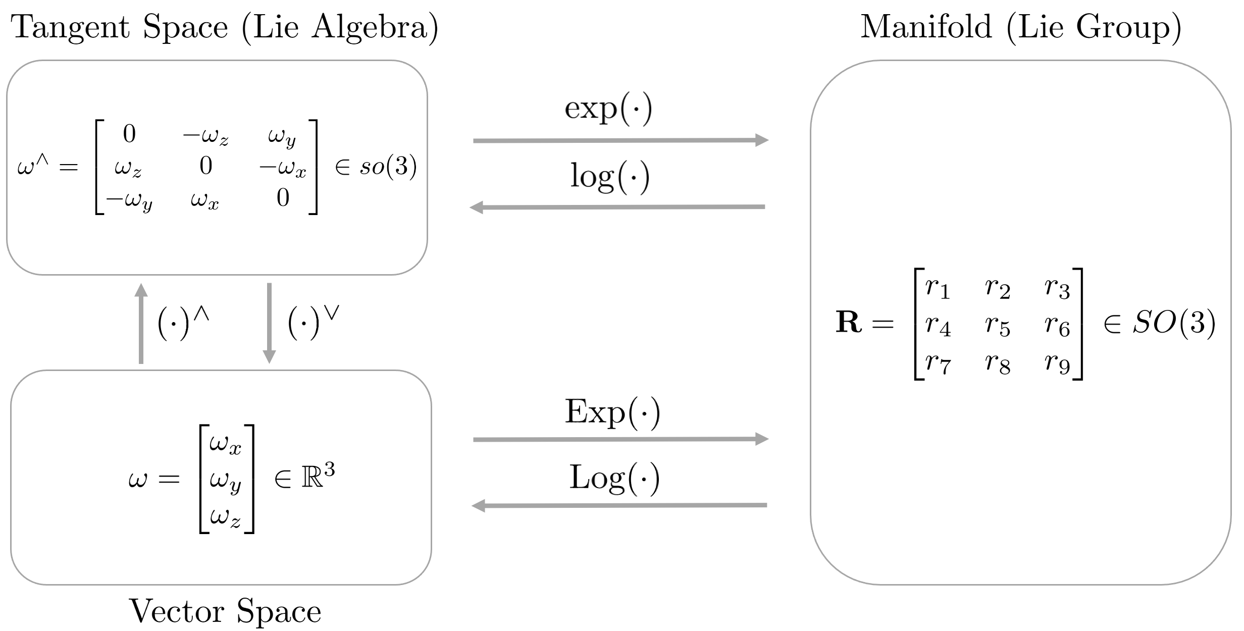
At this time, for the convenience of operation, generally, the $\exp(\cdot)$ operator is used in the process of mapping with $\omega^{\wedge} \rightarrow \mathbf{R}$, and the $\text{Exp}(\cdot)$ operator is used in the process of mapping with $\omega \rightarrow \mathbf{R}$. Logarithm mapping is also the same.
\begin{equation}
\begin{aligned}
\exp(\cdot) & : \omega^{\wedge} \mapsto \mathbf{R} \\
\text{Exp}(\cdot) & : \omega \mapsto \mathbf{R}
\end{aligned}
\end{equation}
If this is summarized in a figure, it is as follows.
Derivation of Exponential Mapping
Any rotation matrix satisfies the following properties.
\begin{equation}
\begin{aligned}
\mathbf{R}^{\intercal}\mathbf{R} = \mathbf{I}
\end{aligned}
\end{equation}
Looking at $\mathbf{R}$ as the camera rotation that continuously changes over time, it can be expressed as a function of time $\mathbf{R}(t)$.
\begin{equation}
\begin{aligned}
\mathbf{R}^{\intercal}(t)\mathbf{R}(t) = \mathbf{I}
\end{aligned}
\end{equation}
Performing the derivative with respect to time on both sides of the above expression gives:
\begin{equation}
\begin{aligned}
& \dot{\mathbf{R}}^{\intercal}(t)\mathbf{R}(t) + \mathbf{R}^{\intercal}(t)\dot{\mathbf{R}}(t) = 0 \\
& \mathbf{R}^{\intercal}(t)\dot{\mathbf{R}}(t) = -\biggl( \mathbf{R}^{\intercal}(t)\dot{\mathbf{R}}(t) \biggl)^{\intercal}
\end{aligned}
\end{equation}
From this, it can be seen that $\mathbf{R}^{\intercal}(t)\dot{\mathbf{R}}(t)$ satisfies the property of an skew-symmetric matrix. Any skew-symmetric matrix $\mathbf{A}$ is as follows. The operator that converts an arbitrary three-dimensional vector $\mathbf{a}$ to $\mathbf{A}$ is defined as $(\cdot)^\wedge$, and the operator that goes in the opposite direction is defined as $(\cdot)^\vee$.
\begin{equation}
\begin{aligned}
\mathbf{a}^{\wedge} = \mathbf{A} = \begin{bmatrix}
0 & -a_{3} & a_{2} \\
a_{3} & 0 & -a_{1} \\
-a_{2} & a_{1} & 0
\end{bmatrix}, \ \ \mathbf{A}^{\vee} = \mathbf{a} = \begin{bmatrix} a_{1} \\ a_{2} \\ a_{3} \end{bmatrix}
\end{aligned}
\end{equation}
For any skew-symmetric matrix, you can find the corresponding vector. So $\mathbf{R}^{\intercal}(t)\dot{\mathbf{R}}(t)$ also corresponds to the 3D vector $\omega(t) \in \mathbb{R}^{ 3}$ can be found.
\begin{equation}
\begin{aligned}
\mathbf{R}^{\intercal}(t)\dot{\mathbf{R}}(t)= \omega(t)^{\wedge}.
\end{aligned}
\end{equation}
At this time, the left side of the equation is multiplied by $\mathbf{R}(t)$. Since $\mathbf{R}(t)$ is an orthogonal matrix, the following expression can be obtained.
\begin{equation}
\begin{aligned}
\dot{\mathbf{R}}(t) = \mathbf{R}(t)\omega(t)^{\wedge} = \mathbf{R}(t)\begin{bmatrix}
0 & -\omega_{z} & \omega_{y} \\
\omega_{z} & 0 & -\omega_{x} \\
-\omega_{y} & \omega_{x} & 0
\end{bmatrix}
\end{aligned}
\end{equation}
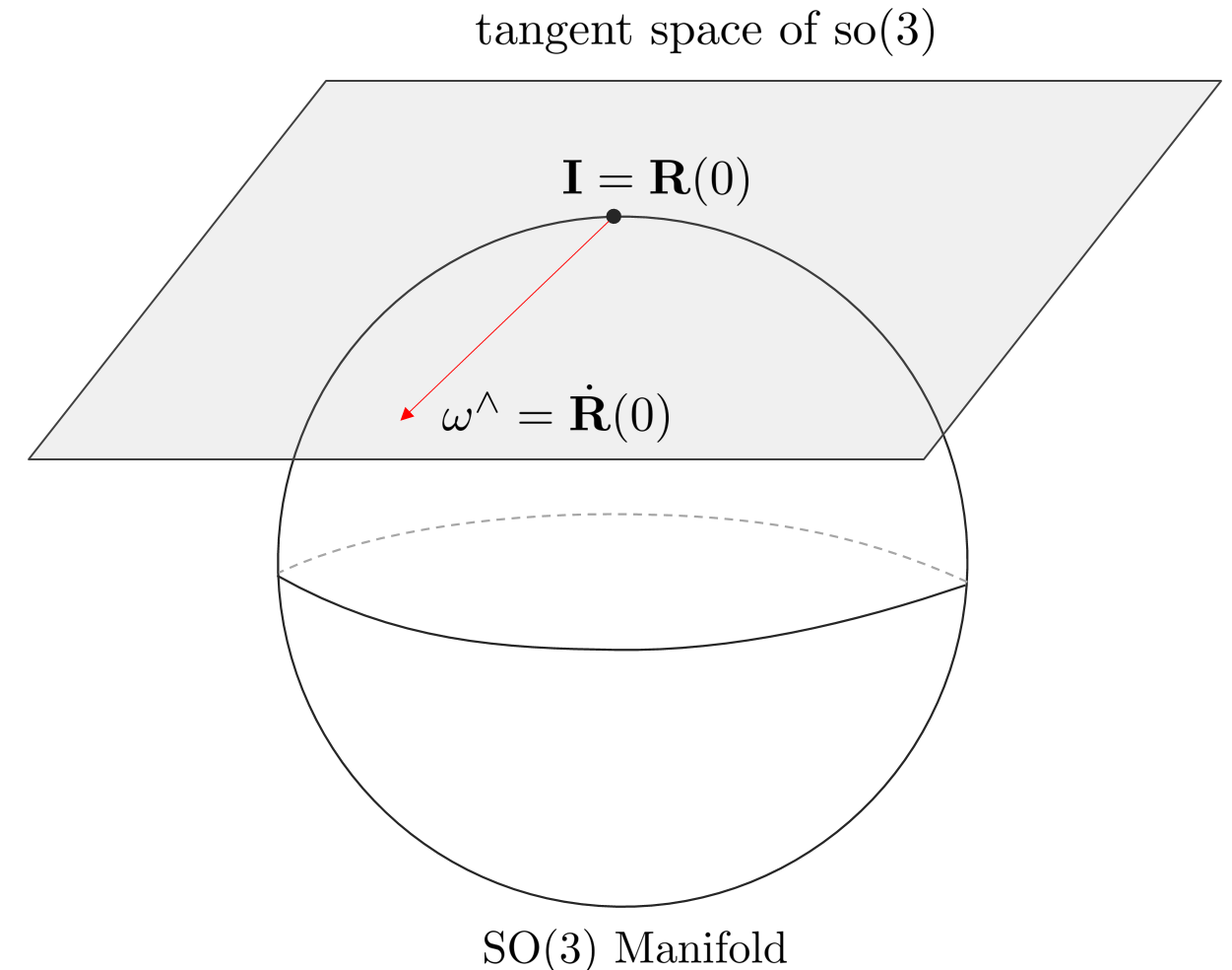
If the rotation matrix $\mathbf{R}(0)=\mathbf{I}$ at time $t_{0}=0$, then $\dot{\mathbf{R}}(0)$ is can indicate
$$\dot{\mathbf{R}}(0) = \omega(0)^{\wedge}$$
At this time, $\omega$ means the tangent plane to the origin of SO(3). Assuming that $\omega$ is constant around $t_{0}=0$, then $\omega(t_{0}) = \omega$.
\begin{equation}
\begin{aligned}
\dot{\mathbf{R}}(t) = \omega(0)^{\wedge} = \omega^{\wedge}
\end{aligned}
\end{equation}
Since the above equation is a differential equation, the solution of the differential equation is:
\begin{equation}
\begin{aligned}
\mathbf{R}(t) = \mathbf{R}_{0}\exp(\omega^{\wedge}t).
\end{aligned}
\end{equation}
if $\mathbf{R}_{0} = \mathbf{R}(0) = \mathbf{I}$ is set and the function expression for time is omitted and expressed as $\omega^{\wedge}t \rightarrow \omega^{\wedge}$, it is as follows.
\begin{equation}
\begin{aligned}
\mathbf{R} = \exp(\omega^{\wedge}).
\end{aligned}
\end{equation}
The above expression means that the rotation matrix can be calculated through $\exp(\omega^{\wedge})$.
Plus and Minus Operator of SO(3)
Using the exponential mapping described so far, $\mathbf{R}$ can be transformed using the angular velocity $\omega$. At this time, since general $+,-$ operators are not applied between SO(3) groups, new $\oplus, \ominus$ operators must be defined. First, the $\oplus$ operator applies an additional rotation by $\omega$ to an arbitrary rotation matrix $\mathbf{R}$.
$$\oplus : SO(3) \times \mathbb{R}^{3} \mapsto SO(3)$$
$$\mathbf{R} \oplus w \triangleq \mathbf{R} \cdot \text{Exp}(\omega)$$
Conversely, the $\ominus$ operator is used together with $\mathbf{R}_{2} \ominus \mathbf{R}_{1}$ when there are two rotation matrices $\mathbf{R}_{1}, \mathbf{R}_{2}$, and it means the difference in rotation between $\mathbf{R}_{1}$ and $\mathbf{R}_{2}$.
$$\ominus : SO(3) \times SO(3) \mapsto \mathbb{R}^{3}$$
$$\mathbf{R}_{2} \ominus \mathbf{R}_{1} \triangleq \text{Log}(\mathbf{R}_{1}^{-1}\mathbf{R}_{2})$$
Adjoint Matrix of SO(3)
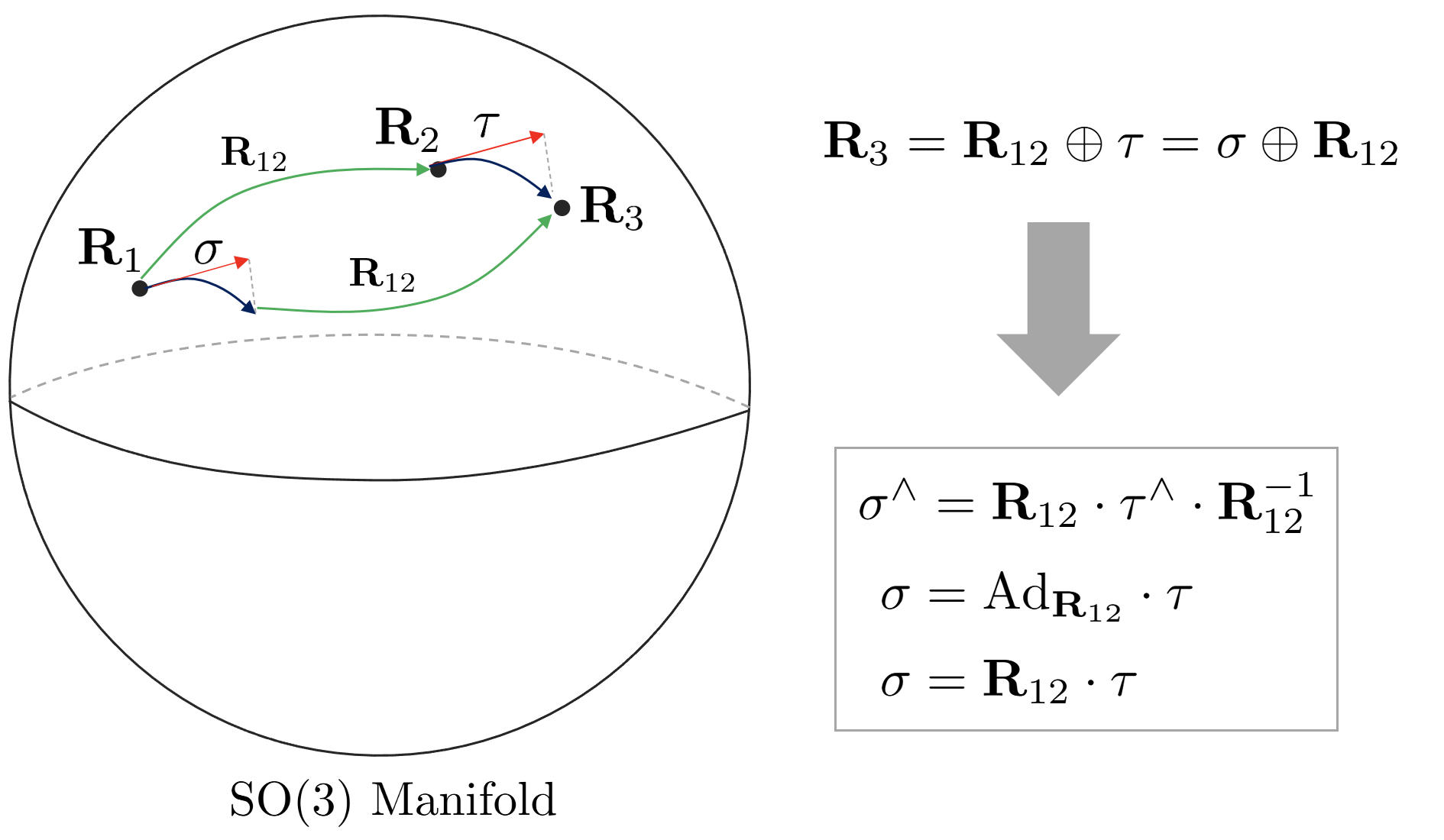
The adjoint matrix of the SO(3) group is a matrix that converts an arbitrary angular velocity $\tau \in \mathbb{R}^{3}$을 다른 $\mathbf{R}_{1}$ existing on a tangent plane of an arbitrary $\mathbf{R}_{2} \in SO(3)$ to an angular velocity $\sigma$ corresponding to another tangent plane of $\mathbf{R}_{1}$. In other words, when there are two Orientation $\mathbf{R}_{1}, \mathbf{R}_{2} \in SO(3)$, the specific angular velocity $\tau$ seen from $\mathbf{R}_{2}$ is converted to the angular velocity $\sigma$ seen from $\mathbf{R}_{1}$ use it when you want to If the adjoint matrix for $\mathbf{R}_{12} \in SO(3)$ is $\text{Ad}_{\mathbf{R}_{12}}$, the following holds.
\begin{equation}
\begin{aligned}
\sigma = \text{Ad}_{\mathbf{R}_{12}}\tau
\end{aligned}
\end{equation}
Since it is a matrix that converts angular velocity $\tau \in \mathbb{R}^{3}$ to another angular velocity $\sigma$, it has the size of $\text{Ad}_{\mathbf{R}_{12}} \in \mathbb{R}^{3\times 3}$. Also, the adjoint matrix satisfies the following formula.
\begin{equation}
\begin{aligned}
& \mathbf{R}_{12}\cdot \exp(\tau^{\wedge}) = \exp((\text{Ad}_{\mathbf{R}_{12}}\cdot \tau)^{\wedge}) \cdot \mathbf{R}_{12} \\
& \exp((\text{Ad}_{\mathbf{R}_{12}}\cdot \tau)^{\wedge}) = \mathbf{R}_{12}\cdot \exp(\tau^{\wedge})\cdot \mathbf{R}_{12}^{-1}
\end{aligned}
\end{equation}
The process of deriving the adjoint matrix for so(3) algebra is as follows.
\begin{equation}
\begin{aligned}
(\text{Ad}_{\mathbf{R}_{12}}\cdot \tau)^{\wedge} & = \mathbf{R}_{12} \cdot \bigg( \sum_{i=1}^{3}\tau_{i}G_{i} \bigg) \cdot \mathbf{R}_{12}^{-1} \\
& = \mathbf{R}_{12} \cdot \tau^{\wedge} \cdot \mathbf{R}_{12}^{-1} \\
& = (\mathbf{R}_{12}\tau)^{\wedge} \\
\end{aligned}
\end{equation}
\begin{equation}
\begin{aligned}
\text{Ad}_{\mathbf{R}_{12}} = \mathbf{R}_{12} \in \mathbb{R}^{3\times 3}
\end{aligned}
\end{equation}
SE(3) Group
Lie Group SE(3)
The Special Euclidean 3 (SE(3)) group, which is one of the Lie groups, means a group consisting of matrices related to the transformation of rigid bodies in 3-dimensional space and closed operations.\begin{equation}
\begin{aligned}
SE(3) = \left \{ \mathbf{T} =
\begin{bmatrix}
\mathbf{R} & \mathbf{t} \\
\mathbf{0} & 1
\end{bmatrix} \in \mathbb{R}^{4\times4} \ | \ \mathbf{R} \in SO(3), \mathbf{t} \in \mathbb{R}^{3} \right \}
\end{aligned}
\end{equation}
The following formula is established for any two conversion matrices $\mathbf{T}_{1}, \mathbf{T}_{2} \in SE(3)$.
\begin{equation}
\begin{aligned}
\mathbf{T}_{1}\mathbf{T}_{2} & = \begin{bmatrix} \mathbf{R}_{1} & \mathbf{t}_{1} \\ \mathbf{0} & 1 \end{bmatrix} \cdot \begin{bmatrix} \mathbf{R}_{2} & \mathbf{t}_{2} \\ \mathbf{0} & 1 \end{bmatrix} \\
& = \begin{bmatrix} \mathbf{R}_{1}\mathbf{R}_{2} & \mathbf{R}_{1}\mathbf{t}_{2} + \mathbf{t}_{1} \\ \mathbf{0} & 1 \end{bmatrix}
\end{aligned}
\end{equation}
The inverse matrix is
\begin{equation}
\begin{aligned}
\mathbf{T}^{-1} = \begin{bmatrix} \mathbf{R}^{T} & -\mathbf{R}^{T}\mathbf{t} \\ \mathbf{0} & 1\end{bmatrix}
\end{aligned}
\end{equation}
Also, for a point or vector $\mathbf{x} = \begin{pmatrix} x&y&z&w \end{pmatrix}^{T} \in \mathbb{P}^{3}$ in $\mathbb{P}^{3}$ Projective Space, the following operation holds.
\begin{equation}
\begin{aligned}
\mathbf{T}\cdot \mathbf{x} & = \begin{bmatrix} \mathbf{R}&\mathbf{t}\\\mathbf{0}&1 \end{bmatrix} \cdot \mathbf{x} \\
& = \begin{bmatrix} \mathbf{R}(x,\ y,\ z)^{T} + w \mathbf{t} \\ w \end{bmatrix}
\end{aligned}
\end{equation}
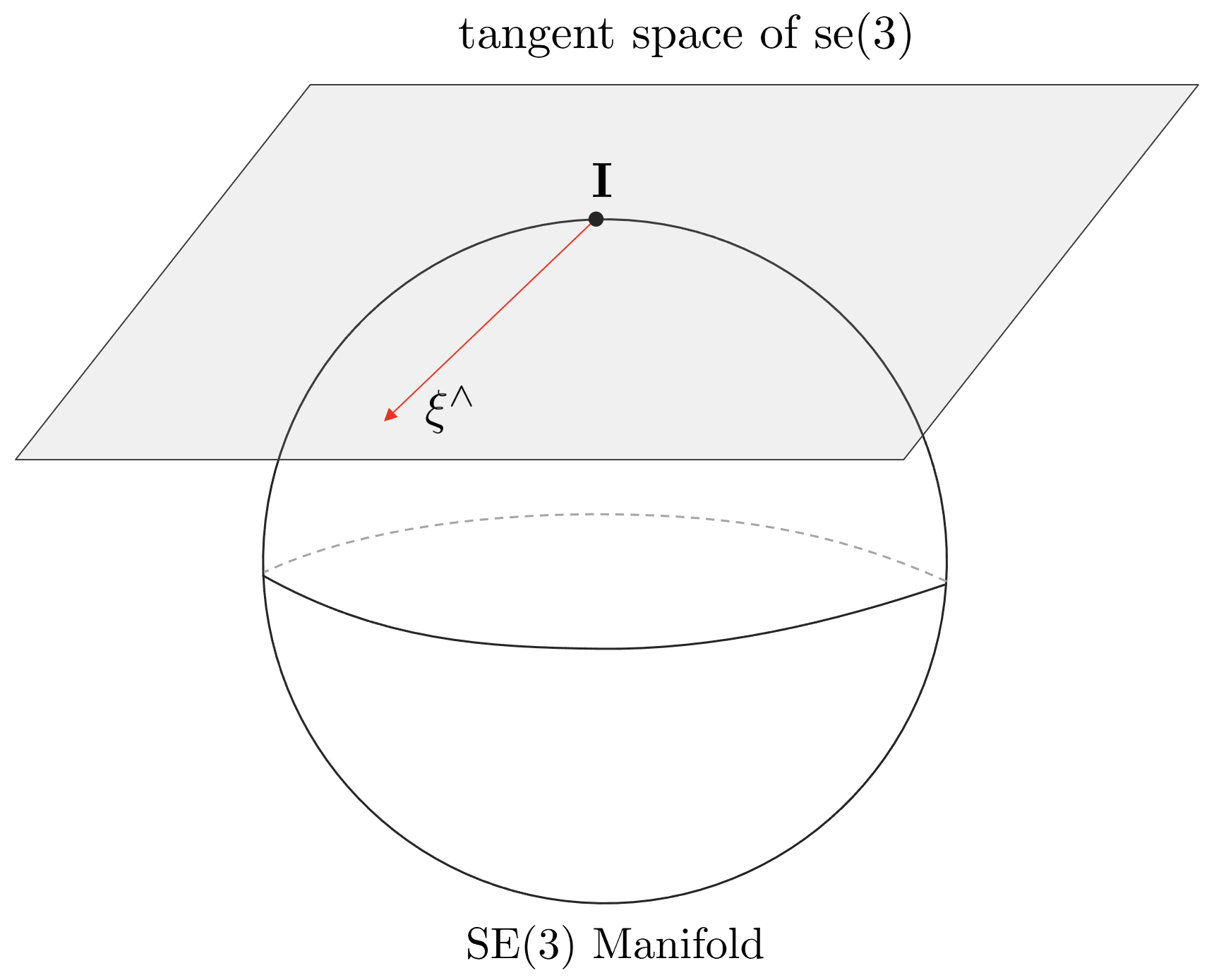
Lie Algebra se(3)
Lie algebra se(3) of the SE(3) group is defined as the following matrix of size $\mathbb{R}^{4\times4}$.
\begin{equation}
\begin{aligned}
\text{se}(3) = \{ \ \xi^{\wedge} = \begin{bmatrix}
\omega^{\wedge} & \mathbf{v} \\
\mathbf{0} & 0
\end{bmatrix} \in \mathbb{R}^{4 \times 4} \ | \ \xi = \begin{bmatrix} \omega \\ \mathbf{v} \end{bmatrix} \in \mathbb{R}^{6} \}
\end{aligned}
\end{equation}
At this time, $\xi$ is twist, meaning the speed of the object in 3D space, and $\omega = \begin{pmatrix} w_{x}&w_{y}&w_{z} \end{pmatrix}^{T} \in \mathbb{R}^{3}$ means angular velocity and $\mathbf{v} = \begin{pmatrix} v_{x}&v_{y}&v_{z} \end{pmatrix}^{T} \in \mathbb{R}^{3}$ means speed. The order of $\omega$ and $\mathbf{v}$ in $\xi$ is often interchanged.
se(3) has 6 generators related to orientation and translation as follows.\begin{equation}
\begin{aligned}
& G_{1} = \begin{pmatrix} 0&0&0&0 \\ 0&0&-1&0 \\ 0&1&0&0 \\ 0&0&0&0 \end{pmatrix}, \ \ G_{2} = \begin{pmatrix} 0&0&1&0 \\ 0&0&0&0 \\ -1&0&0&0 \\ 0&0&0&0 \end{pmatrix},\ \ G_{3} = \begin{pmatrix} 0&-1&0&0 \\ 1&0&0&0 \\ 0&0&0&0 \\ 0&0&0&0 \end{pmatrix} \\
& G_{4} = \begin{pmatrix} 0&0&0&1 \\ 0&0&0&0 \\ 0&0&0&0 \\ 0&0&0&0 \end{pmatrix}, \ \ G_{5} = \begin{pmatrix} 0&0&0&0 \\ 0&0&0&1 \\ 0&0&0&0 \\ 0&0&0&0 \end{pmatrix},\ \ G_{6} = \begin{pmatrix} 0&0&0&0 \\ 0&0&0&0 \\ 0&0&0&1 \\ 0&0&0&0 \end{pmatrix} \\
\end{aligned}
\end{equation}
Each element of se(3) can be expressed as a linear combination of constructors.
\begin{equation}
\begin{aligned}
& \xi = (\omega,\ \mathbf{v})^{T} \in \mathbb{R}^{6} \\
& \omega_{1}G_{1} + \omega_{2}G_{2} + \omega_{3}G_{3} + v_{1}G_{4} + v_{2}G_{5} + v_{3}G_{6} \in se(3)
\end{aligned}
\end{equation}
Exponential Mapping and Logarithm Mapping
Lie Group SE(3) and Lie Algebra se(3) are characterized by one-to-one matching with exponential mapping and logarithm mapping. First of all, the operation $\xi^{\wedge}$ that converts twist $\xi \in \mathbb{R}^{6}$ to se(3) lie algebra is defined as follows.
\begin{equation}
\begin{aligned}
\xi^{\wedge} = \begin{bmatrix} \omega^{\wedge} & \mathbf{v} \\ \mathbf{0} & 0 \end{bmatrix} \in \mathbb{R}^{4\times 4}
\end{aligned}
\end{equation}
The exponential mapping of se(3) is defined as follows.
\begin{equation}
\begin{aligned}
\exp(\xi^{\wedge}) & = \exp \begin{bmatrix} \omega^{\wedge} & \mathbf{v} \\ \mathbf{0} & 0 \end{bmatrix} \\
& = \mathbf{I} + \begin{bmatrix} \omega^{\wedge} & \mathbf{v} \\ \mathbf{0} & 0 \end{bmatrix} + \frac{1}{2!} \begin{bmatrix} (\omega^{\wedge})^{2} & \omega^{\wedge}\mathbf{v} \\ \mathbf{0} & 0 \end{bmatrix} + \frac{1}{3!} \begin{bmatrix} (\omega^{\wedge})^{3} & (\omega^{\wedge})^{2}\mathbf{v} \\ \mathbf{0} & 0 \end{bmatrix} + \cdots
\end{aligned}
\end{equation}
At this time, the part related to rotation is the same as the SO (3) group, but the part related to movement has a separate series form.
\begin{equation}
\begin{aligned}
\exp \begin{bmatrix} \omega^{\wedge} & \mathbf{v} \\ \mathbf{0} & 0 \end{bmatrix} & = \begin{bmatrix} \sum_{0}^{\infty}\frac{1}{n!}(\omega^{\wedge})^{n} & \sum_{0}^{\infty}\frac{1}{(n+1)!}(\omega^{\wedge})^{n} \mathbf{v} \\ \mathbf{0} & 0 \end{bmatrix} \\
& = \begin{bmatrix} \exp(\omega^{\wedge}) & \mathbf{Qv} \\ \mathbf{0} & 1 \end{bmatrix}
\end{aligned}
\end{equation}
\begin{equation}
\begin{aligned}
\mathbf{Q} = \mathbf{I} + \frac{1}{2!}\omega^{\wedge} + \frac{1}{3!}(\omega^{\wedge})^{2} + \frac{1}{4!}(\omega^{\wedge})^{3} + \frac{1}{5!}(\omega^{\wedge})^{4} + \cdots
\end{aligned}
\end{equation}
Applying the principle of the Rodrigues formula and the skew-symmetric matrix explained in the SO (3) part above, it is rearranged as follows.
\begin{equation}
\begin{aligned}
\mathbf{Q} & = \mathbf{I} + \frac{1}{2!}\omega^{\wedge} + \frac{1}{3!}(\omega^{\wedge})^{2} + \frac{1}{4!}(\omega^{\wedge})^{3} + \frac{1}{5!}(\omega^{\wedge})^{4} + \cdots \\
& = \mathbf{I} + \bigg( \frac{1}{2!} - \frac{\theta^{2}}{4!} + \frac{\theta^{4}}{6!} + \cdots \bigg) \omega^{\wedge} + \bigg( \frac{1}{3!} - \frac{\theta^{2}}{5!} + \frac{\theta^{4}}{7!} + \cdots \bigg) (\omega^{\wedge})^{2} \\
& = \mathbf{I} + \sum_{i=0}^{\infty} \begin{bmatrix} \frac{(\omega^{\wedge})^{2i+1}}{(2i+2)!} + \frac{(\omega^{\wedge})^{2i+2}}{(2i+3)!} \end{bmatrix} \\
& = \mathbf{I} + \bigg(\sum_{i=0}^{\infty} \frac{(-1)^{i}\theta^{2i}}{(2i+2)!} \bigg) \omega^{\wedge} + \bigg( \sum_{i=0}^{\infty}\frac{(-1)^{i}\theta^{2i}}{(2i+3)!} \bigg) (\omega^{\wedge})^{2} \\
& = \mathbf{I} + \bigg( \frac{1-\cos\theta}{\theta^{2}} \bigg) \omega^{\wedge} + \bigg(\frac{\theta-\sin\theta}{\theta^{3}} \bigg) (\omega^{\wedge})^{2}
\end{aligned}
\end{equation}
Summarizing the derivation process so far, the exponential mapping of se(3) is expressed as follows.
\begin{equation}
\begin{aligned}
& \xi = (\omega, \mathbf{v}) \in \mathbb{R}^{6} \\
& \theta = |\omega| \\
& \theta^{2} = \omega^{\intercal}\omega \\
& A = \frac{\sin\theta}{\theta} \\
& B = \frac{1-\cos\theta}{\theta^{2}} \\
& C = \frac{1-A}{\theta^{2}} = \frac{\theta - \sin\theta}{\theta^{3}} \\
& \mathbf{R} = \mathbf{I} + A\omega^{\wedge} + B (\omega^{\wedge})^{2} \\
& \mathbf{Q} = \mathbf{I} + B\omega^{\wedge} + C (\omega^{\wedge})^{2} \\
\end{aligned}
\end{equation}
\begin{equation}
\begin{aligned}
\exp(\xi^{\wedge}) = \begin{bmatrix} \mathbf{R} & \mathbf{Qv} \\ \mathbf{0} & 1 \end{bmatrix}
\end{aligned}
\end{equation}
The log mapping of the SE(3) group uses the log mapping of the SO(3) group for the rotating part and $\mathbf{Q}^{-1}$ for the moving part.
\begin{equation}
\begin{aligned}
& \mathbf{Q}^{-1} = \mathbf{I} - \frac{1}{2!}\omega^{\wedge} + \frac{1}{\theta^{2}} \bigg( 1 - \frac{A}{2B} \bigg) (\omega^{\wedge})^{2} \\
\end{aligned}
\end{equation}
\begin{equation}
\begin{aligned}
& \omega^{\wedge} = \log(\mathbf{R}) \\
& \mathbf{v} = \mathbf{Q}^{-1}\mathbf{t}
\end{aligned}
\end{equation}
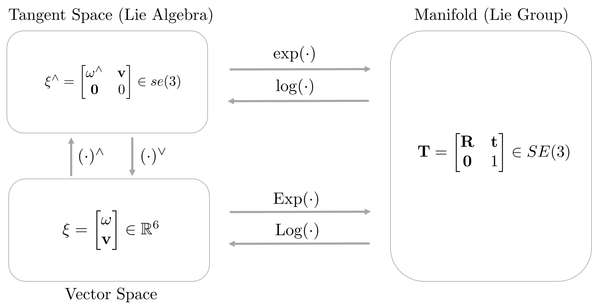
As with SO(3), for the convenience of operation, the process of mapping to $\xi^{\wedge} \rightarrow \mathbf{T}$ generally uses the $\exp(\cdot)$ operator, and the process of mapping to $\xi\rightarrow \mathbf{T}$ uses the $\text{Exp}(\cdot)$ operator make use of Logarithm mapping is also the same.
\begin{equation}
\begin{aligned}
\exp(\cdot) & : \xi^{\wedge} \mapsto \mathbf{T} \\
\text{Exp}(\cdot) & : \xi \mapsto \mathbf{T}
\end{aligned}
\end{equation}
If this is summarized in a figure, it is as follows.
Plus and Minus Operator of SE(3)
Using the exponential mapping described so far, $\mathbf{T}$ can be converted using twist $\xi$. At this time, like SO(3), common $+,-$ operators are not applied between SE(3) groups, so new $\oplus$ and $\ominus$ operators must be defined. First of all, the $\oplus$ operator applies an additional transformation as much as $\xi$ to an arbitrary pose $\mathbf{T}$.
$$\mathbf{T} \oplus \xi \triangleq \mathbf{T} \cdot \text{Exp}(\xi)$$
Conversely, the $\ominus$ operator is used with $\mathbf{T}_{2} \ominus \mathbf{T}_{1}$ when two poses $\mathbf{T}_{1}, \mathbf{T}_{2}$ exist, and means the relative pose of $\mathbf{T}_{1}$ to $\mathbf{T}_{2}$.
$$\mathbf{T}_{2} \ominus \mathbf{T}_{1} \triangleq \text{Log}(\mathbf{T}_{1}^{-1}\mathbf{T}_{2})$$
Adjoint Matrix of SE(3)
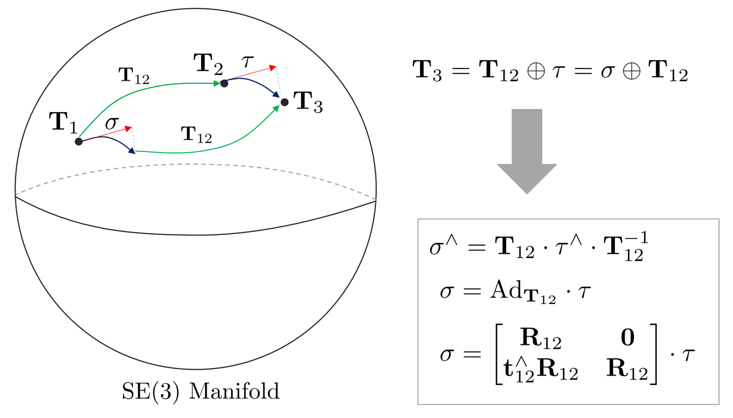
The adjoint matrix of the SE(3) group is a matrix that converts an arbitrary twist $\tau \in \mathbb{R}^{6}$ existing on the tangent plane of an arbitrary $\mathbf{T}_{2} \in SE(3)$ to a twist $\sigma$ corresponding to the tangent plane of another $\mathbf{T}_{1}$. In other words, when there are two Pose $\mathbf{T}_{1}, \mathbf{T}_{2} \in SE(3)$, it is used to convert the specific twist $\tau$ seen from $\mathbf{T}_{2}$ to twist $\sigma$ seen from $\mathbf{T}_{1}$. If the adjoint matrix for $\mathbf{T}_{12} \in SE(3)$ is $\text{Ad}_{\mathbf{T}_{12}}$, the following holds.
\begin{equation}
\begin{aligned}
\xi_{1} = \text{Ad}_{\mathbf{T}_{12}}\xi_{2}
\end{aligned}
\end{equation}
Since it is a matrix that transforms a twist into another twist, it has a size of $\text{Ad}_{\mathbf{T}_{12}} \in \mathbb{R}^{6\times 6}$. Also, the adjoint matrix satisfies the following formula.
\begin{equation}
\begin{aligned}
&\mathbf{T}_{12} \cdot \exp(\tau^{\wedge}) = \exp((\text{Ad}_{\mathbf{T}_{12}}\cdot \tau)^{\wedge})\cdot \mathbf{T}_{12} \\
&\exp((\text{Ad}_{\mathbf{T}_{12}}\cdot \tau)^{\wedge}) = \mathbf{T}_{12}\cdot \exp(\tau^{\wedge})\cdot \mathbf{T}_{12}^{-1}
\end{aligned}
\end{equation}
The derivation process of the Adjoint matrix for se(3) algebra is as follows.
\begin{equation}
\begin{aligned}
(\text{Ad}_{\mathbf{T}_{12}}\cdot \tau)^{\wedge} & = \mathbf{T}_{12} \cdot \bigg( \sum_{i=1}^{6}\xi_{i}G_{i} \bigg) \cdot \mathbf{T}_{12}^{-1} \\
& = \begin{pmatrix} \mathbf{R}_{12}\omega_{12} \\ \mathbf{t}_{12}^{\wedge}\mathbf{R}_{12}\omega_{12} + \mathbf{R}_{12}\mathbf{v}_{12} \end{pmatrix}^{\wedge} \\
& = \bigg(\begin{pmatrix} \mathbf{R}_{12} & \mathbf{0} \\ \mathbf{t}_{12}^{\wedge}\mathbf{R}_{12} & \mathbf{R}_{12} \end{pmatrix} \begin{pmatrix} \omega_{12} \\\mathbf{v}_{12} \end{pmatrix} \bigg)^{\wedge}
\end{aligned}
\end{equation}
\begin{equation}
\begin{aligned}
\text{Ad}_{\mathbf{T}_{12}} = \begin{bmatrix} \mathbf{R}_{12} & \mathbf{0} \\ \mathbf{t}_{12}^{\wedge}\mathbf{R}_{12} & \mathbf{R}_{12} \end{bmatrix} \in \mathbb{R}^{6\times 6}
\end{aligned}
\end{equation}
Applications for estimation
Next, we look at an example of actual state estimation using Lie Group. Assume that cameras and landmarks exist in a 3D space as shown below.
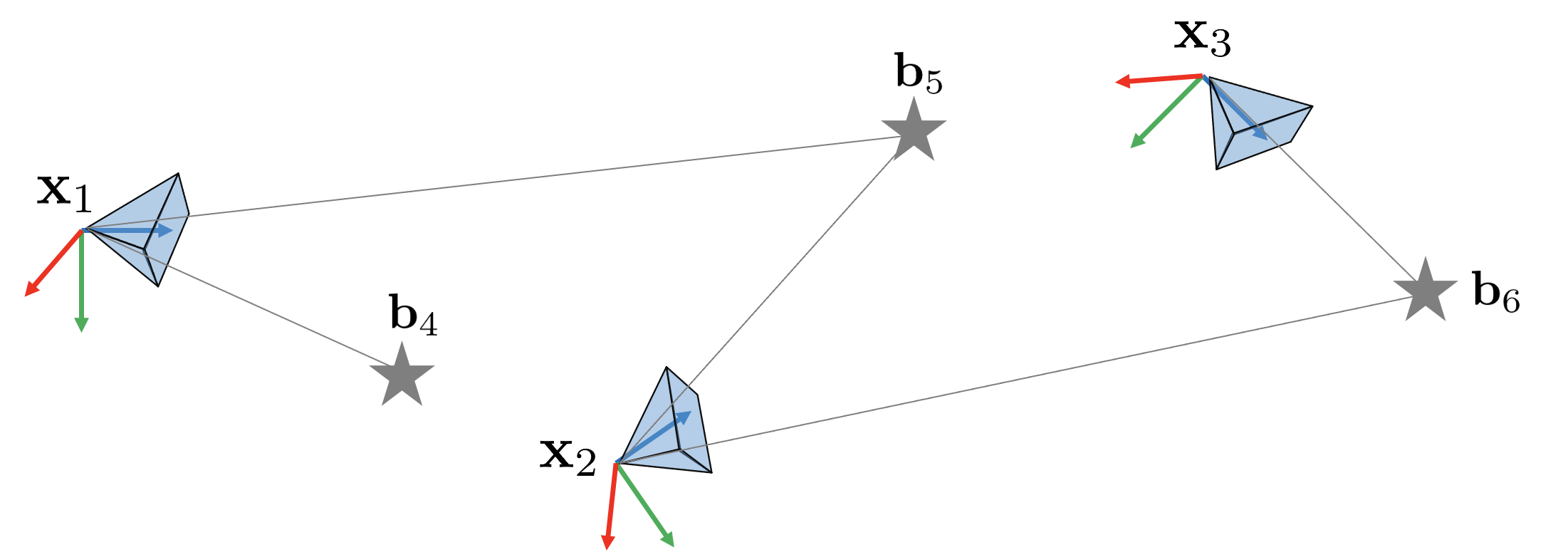
At this time, $\mathbf{x}_{i}, i=1,2,3$ means the pose of the camera in 3D space, and $\mathbf{b}_{i}, i=4,5, 6$ means the coordinates of landmarks.
EKF map-based localzation
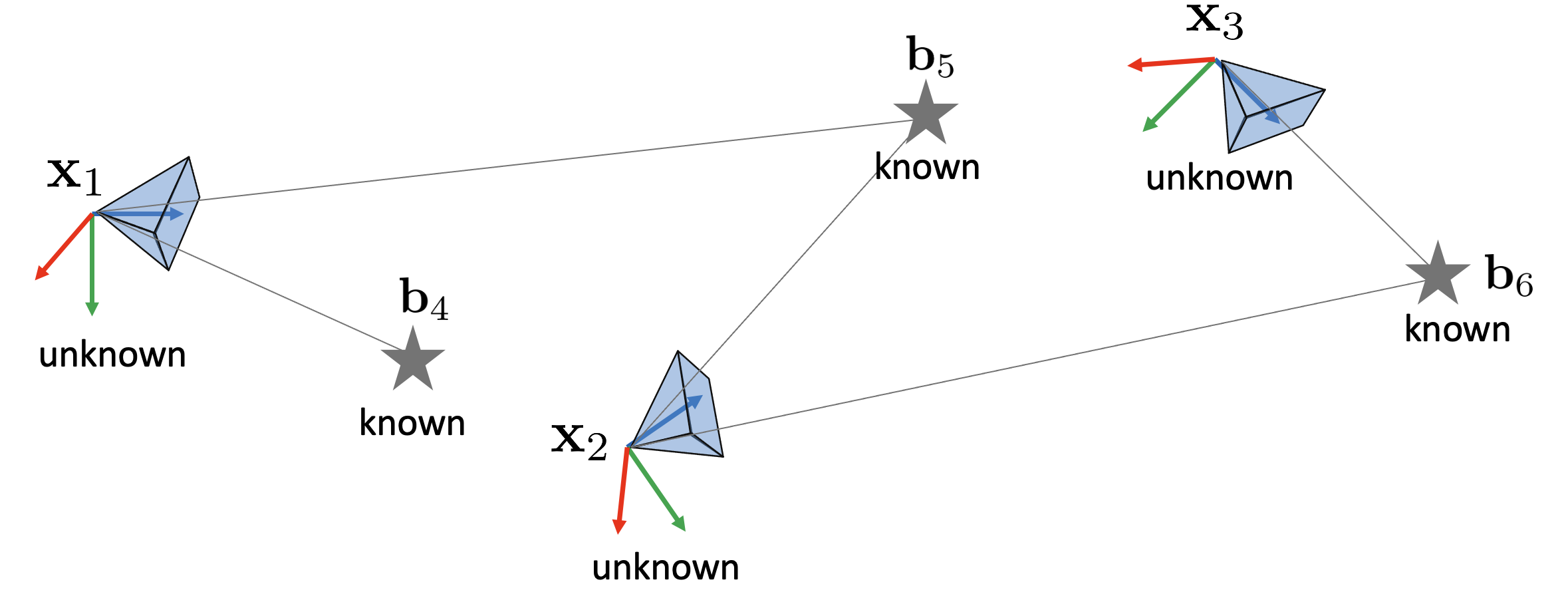
If $\mathbf{x}_{i}$ is not known and only the value of $\mathbf{b}_{i}$ is given, the camera uses the landmark to pose itself $\mathbf{x} _{i}$ can be estimated through EKF.
\begin{equation}
\begin{aligned}
\mathbf{x} \sim \mathcal{N}(\bar{\mathbf{x}}, \mathbf{P}) \in SE(3) & : \text{Unknown} \\
\mathbf{P} = \mathbb{E}[(\mathbf{x} \ominus \bar{\mathbf{x}})(\mathbf{x} \ominus \bar{\mathbf{x}})^{\intercal}] & : \text{Unknown} \\
\mathbf{b} \in \mathbb{R}^{3} &: \text{Known} \\
\end{aligned}
\end{equation}
The motion model and measurement model of the camera are as follows.
\begin{equation}
\begin{aligned}
& \text{motion model: } & \mathbf{x}_{i} & = f(\mathbf{x}_{i-1}, \mathbf{u}_{i}) = \mathbf{x}_{i-1} \oplus (\mathbf{u_{i}}dt + \omega) \\
& \text{measurement model: } & \mathbf{y}_{k} & = h(\mathbf{x}) = \mathbf{x}^{-1}\mathbf{b}_{k} + v, \quad \text{where, } v \sim \mathcal{N}(0, \mathbf{R})
\end{aligned}
\end{equation}
- $\omega \sim \mathcal{N}(0, \mathbf{Q})$ : perturbation
- $v \sim \mathcal{N}(0, \mathbf{R})$ : noise
At this time, since the pose of the camera belongs to the SE (3) group, the pose is updated using the $\oplus$ operation. The prediction and correction steps of EKF using the above two models are as follows
Prediction Step
\begin{equation}
\begin{aligned}
\hat{\mathbf{x}} & \leftarrow \hat{\mathbf{x}} \oplus \mathbf{u}_{i}dt \\
\mathbf{P} & \leftarrow \mathbf{FPF}^{\intercal} + \mathbf{GQG}^{\intercal}
\end{aligned}
\end{equation}
- $\mathbf{F} = \frac{Df}{D\mathbf{x}}$
- $\mathbf{G} = \frac{Df}{D\omega}$
Correction Step
\begin{equation}
\begin{aligned}
\mathbf{z}_{k} & = \mathbf{y}_{k} - \hat{\mathbf{x}}^{-1}\mathbf{b}_{k} \\
\mathbf{Z}_{k} & = \mathbf{HPH}^{\intercal} + \mathbf{R} \\
\mathbf{K} & = \mathbf{PH}^{\intercal}\mathbf{Z}^{-1}_{k} \\
\hat{\mathbf{x}} & \leftarrow \hat{\mathbf{x}} \oplus \mathbf{Kz}_{k} \\
\mathbf{P} & \leftarrow \mathbf{P} - \mathbf{KZ}_{k}\mathbf{K}^{\intercal} \\
\end{aligned}
\end{equation}
- $\mathbf{H} = \frac{Dh}{D\mathbf{x}}$
The above formula is the same as the general EKF formula. Therefore, if the Lie Group operator $\oplus, \ominus, \frac{D*}{D*}, \mathbf{x}^{-1}$ is used, the nonlinear $SE(3)$ operation can be performed identically to the operation used in the linear vector space.
Pose Graph SLAM
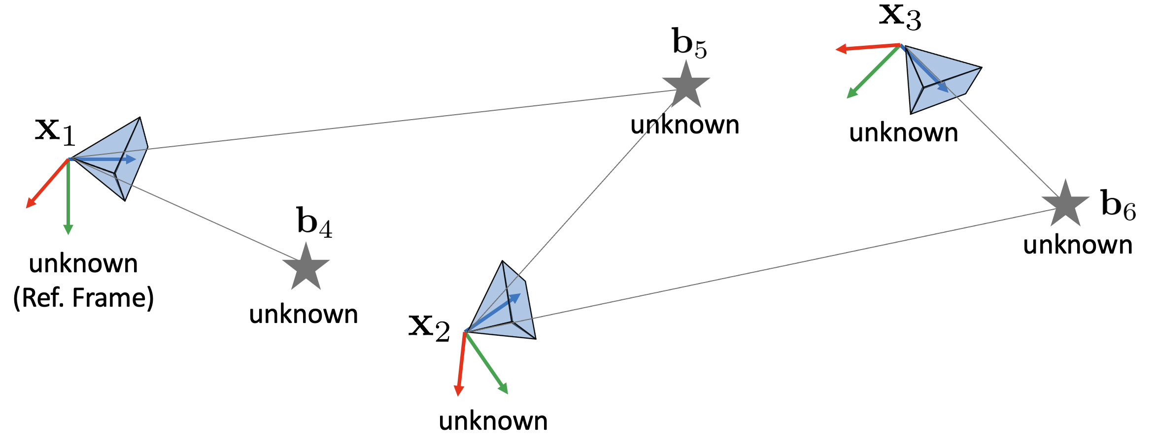
If $\mathbf{x}_{i}$ and $\mathbf{b}_{i}$ are both unknown, then the two state variables can be estimated through pose graph SLAM.\begin{equation}
\begin{aligned}
\mathbf{x} \in SE(3) & : \text{Unknown} \\
\mathbf{b} \in \mathbb{R}^{3} &: \text{Unknown}
\end{aligned}
\end{equation}
At this time, the state variable can be expressed as a vector in a bundle at once as follows.
\begin{equation}
\begin{aligned}
\mathbf{x} = (\mathbf{x}_{1}, \mathbf{x}_{2},\mathbf{x}_{3}, \mathbf{b}_{4}, \mathbf{b}_{5}, \mathbf{b}_{6})
\end{aligned}
\end{equation}
At this time, the nonlinear optimization problem can be defined as follows.
\begin{equation}
\begin{aligned}
\mathbf{x}^{*} = \arg\min_{\mathbf{x}} \sum_{p} \left \| \mathbf{r}_{p}(\mathbf{x}) \right \|^{2}
\end{aligned}
\end{equation}
At this time, the residual $\mathbf{r}$ can be defined as follows.
\begin{equation}
\begin{aligned}
\text{prior: } & \mathbf{r}_{1} = \Omega_{1}^{\intercal/2} (\mathbf{x}_{1} \ominus \mathbf{x}_{1}^{ref}) \\
\text{motion: } & \mathbf{r}_{ij} = \Omega_{ij}^{\intercal/2} (\mathbf{u}_{j}dt - (\mathbf{x}_{j} \ominus \mathbf{x}_{i})) \\
\text{measurement: } & \mathbf{r}_{ik} = \Omega_{ik}^{\intercal/2} (\mathbf{y}_{ik} - \mathbf{x}^{-1}_{i} \mathbf{b}_{k})
\end{aligned}
\end{equation}
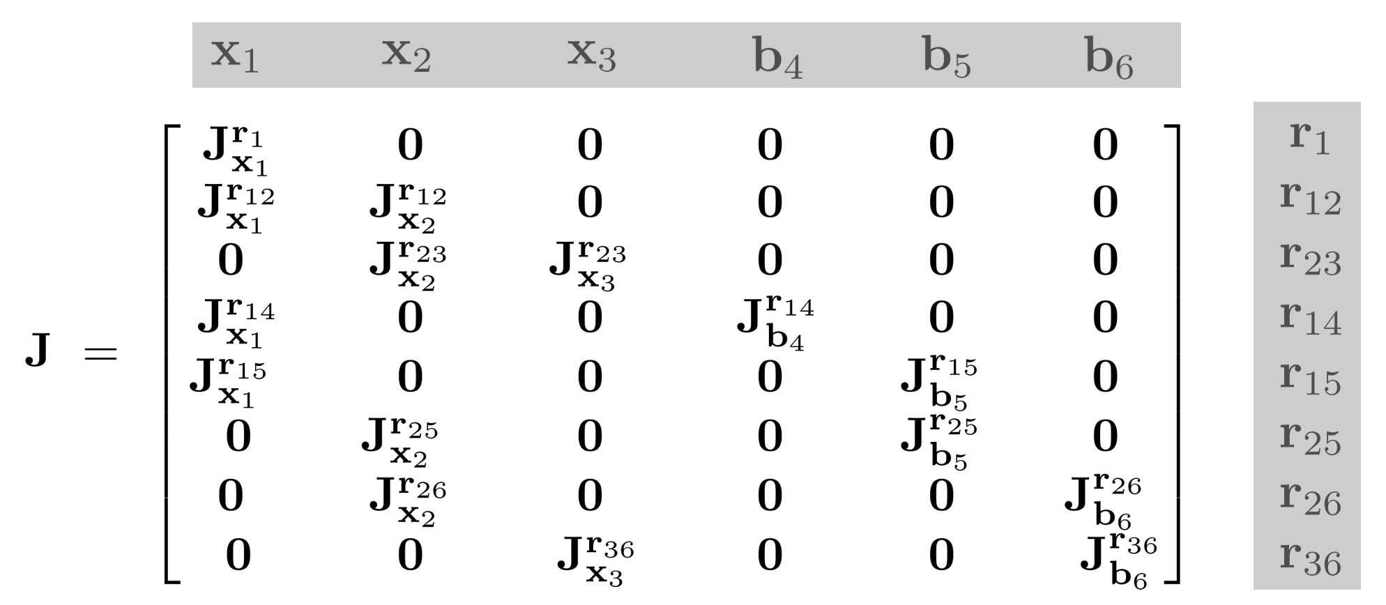
And the residual and Jacobian for all camera poses and landmarks can be defined as follows.
\begin{equation}
\begin{aligned}
\mathbf{r} = \begin{bmatrix} \mathbf{r}_{1} & \mathbf{r}_{12} & \mathbf{r}_{23} & \mathbf{r}_{14} & \mathbf{r}_{15} & \mathbf{r}_{25} & \mathbf{r}_{26} & \mathbf{r}_{36} \end{bmatrix}^{\intercal}
\end{aligned}
\end{equation}
Using the Jacobian above, the nonlinear optimization problem defined above can be solved iteratively through Newton steps.
\begin{equation}
\begin{aligned}
\Delta \mathbf{x} & = -(\mathbf{J}^{\intercal}\mathbf{J})^{-1}\mathbf{J}^{\intercal}\mathbf{r} \\
\mathbf{x} & \leftarrow \mathbf{x} \oplus \Delta \mathbf{x}
\end{aligned}
\end{equation}
In this case, the optimization formula used is also nonlinear $SE(3)$ through Lie Group operators $\oplus, \ominus, \frac{D*}{D*}, \mathbf{x}^{-1}$, etc. The operation can be performed in the same way as the operation used in the linear vector space.
Lie Theory-based Optimization on SLAM
In the Lie Theory-based optimization method, when updating the camera pose in the 3D space, SE(3) must check whether the constraints are violated every time the variation is updated due to its own constraints. However, if the local tangent plane se(3) is used, the change in se(3) is obtained through non-linear optimization and mapped to the SE(3) space through exponential mapping, thereby enabling optimization without constraints.
Therefore, using Lie Theory has the same advantages as converting and solving the existing constrained optimization problem into an unconstrained opotimization problem. In addition, since Lie Algebra se (3) is a linear vector space, it is relatively easy to calculate jacobian and perturbation, so modeling (error, perturbation, etc) for applying existing optimization techniques can be used as it is.
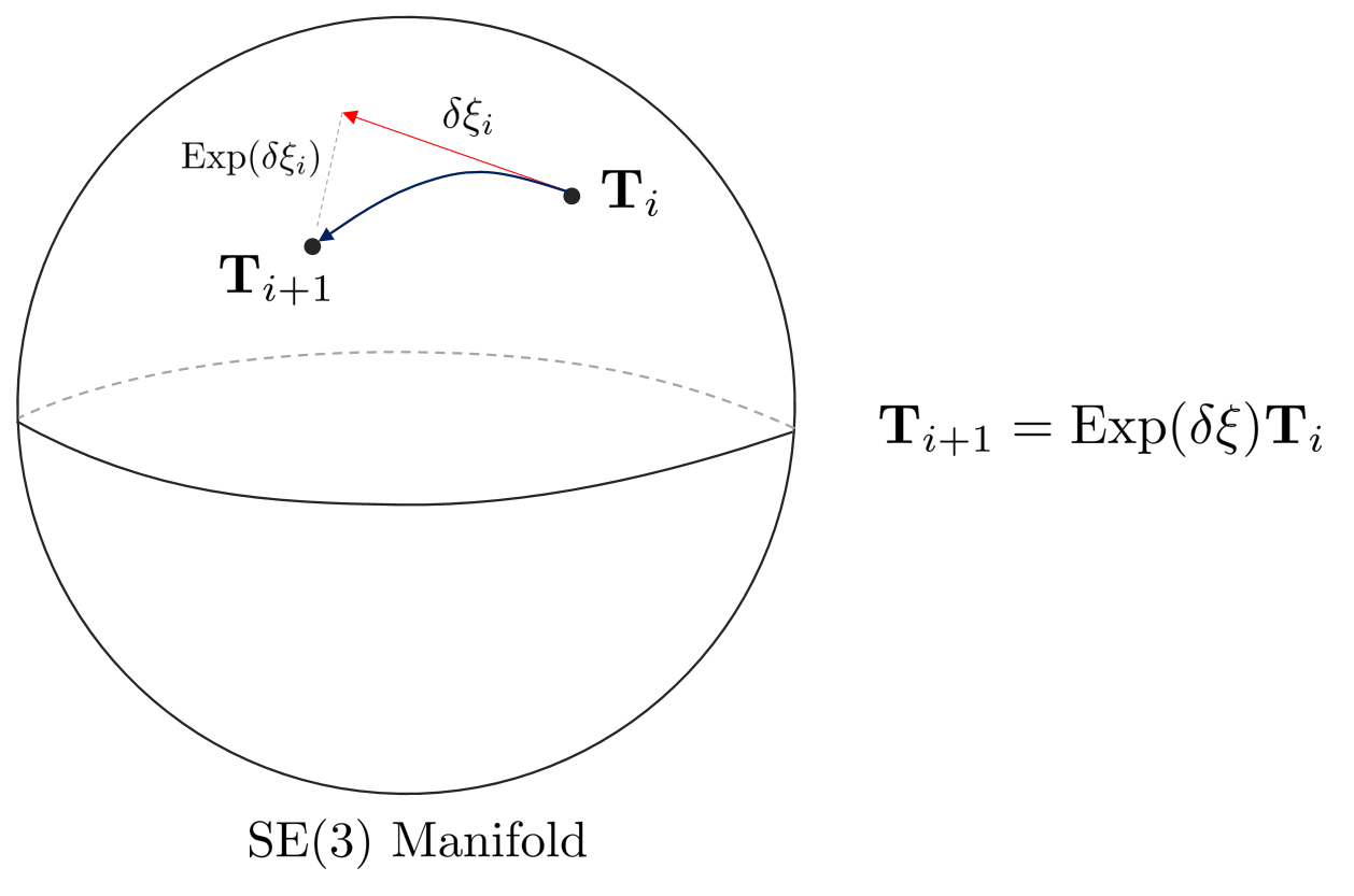
In other words, if non-linear optimization is performed by setting the optimization variable to $\delta \xi = [\delta \omega, \delta \mathbf{v}]^{\intercal}$ in SLAM, the increment calculated for each iteration can be converted into SE(3) group through $\text{Exp}(\delta \xi_{i})$. If you update the pose by multiplying this by the existing camera pose $\mathbf{T}_{i}$, you can proceed with the update without worrying about additional constraints.
\begin{equation}
\begin{aligned}
& \mathbf{T}_{i+1} \leftarrow \text{Exp}(\delta \xi_{i}) \cdot \mathbf{T}_{i}
\end{aligned}
\end{equation}
References
1. [pdf] Lie Groups for 2D and 3D Transformations
2. [pdf] A tutorial on SE3 transformation parameterizations and on-manifold optimization
4. [youtube] Modern Robotics Lecture
5. [blog] [데이터분석] 매니폴드(manifold)란? - greatjoy
6. [youtube] Lie theory for the roboticist (by Joan Sola)
Closure
The pdf version is available soon.
'English' 카테고리의 다른 글
| [SLAM][En] Direct Sparse Odometry (DSO) Paper Review Part 2 (0) | 2023.01.17 |
|---|---|
| [SLAM][En] Direct Sparse Odometry (DSO) Paper Review Part 1 (0) | 2023.01.17 |
| [En] Notes on Plücker Coordinate (0) | 2023.01.17 |
| [SLAM][En] Errors and Jacobian Derivations for SLAM Part 2 (0) | 2023.01.17 |
| [SLAM][En] Errors and Jacobian Derivations for SLAM Part 1 (0) | 2023.01.17 |


