 A L I D A
In this post, we review the DSO paper, which is famous for its direct method-based VO algorithm. While analyzing the DSO code, I found out that there were a lot of details omitted in the thesis, and I wrote a summary that included formula derivation and code review by referring to other people's already well-organized data.
1. Initialization
1.1 Calibration
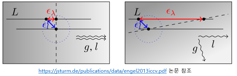
Since the direct method estimates the camera pose by optimizing the brightness error, it is sensitive to the brightness difference of the image. Machine vision cameras, which are mainly used in SLAM, generally automatically adjust the exposure time according to the brightness change of the image (auto exposure), so the direct method may not work normally if the brightness change according to the exposure time is severe. Below is an example of [13] paper.

1.1.1 Photometric Calibration
Therefore, in the DSO paper, a method called photometric calibration was performed along with the geometric calibration generally performed in the VO algorithm. Photometric calibration takes into account camera exposure time, vignetting, camera response function, etc., allowing the direct method to continuously optimize brightness errors. The detailed formula is as follows.
$$\begin{matrix}
I_i(\mathbf{x}) = G(t_iV(\mathbf{x})B_i(\mathbf{x})) \\
I'_i(\mathbf{x}) := t_i B_i(\mathbf{x}) = {G^{-1}(I_i(\mathbf{x})) \over V(\mathbf{x})}
\end{matrix}$$
- $G(\cdot)$ : Response function according to camera exposure time
- $t_{i}$: exposure time
- $V(\cdot)$ : vignetting
- $B(\cdot)$ : irradiance
- $I(\cdot)$ : Observed pixel brightness
- $I^{'}(\cdot)$ : calibrated pixel brightness
For a detailed explanation of $B(\cdot)$, refer to link1, link2. First, the response function $G(\cdot)$ and the irradiance $B(\cdot)$ according to the exposure time of the camera are estimated while applying different exposure times for the same place. The method was prepared by referring to the DSO Photometric Calibration paper

Next, $V(\cdot)$ is estimated. Estimating the pose of the camera by installing the AR marker on the wall, predicting the degree of darkness around the center of the image as a function.

DSO used the image image $I'(\cdot)$, which is relatively invarant to the exposure time change through the above photometric calibration process.

The graph in the middle of the figure above shows the change in exposure time according to the image sequence. Looking at the values, it can be seen that even within the same data, a change in exposure time of up to 500 times or more occurs from 0.018 ms to 10.5 ms. The DSO greatly improved the pose estimation performance of the direct method by calibrating the brightness change according to the camera exposure time change without modeling it as an error function.
1.2 Error Function Formulation

As follows, a point $\mathbf{X}_{1}$ on the 3D space and a point $\mathbf{p}_{1}$ on the 2D image plane have the following relationship.
$$\mathbf{p}_{1} = \pi(\mathbf{X_{1}}) = \mathbf{K}\rho_{1}\mathbf{X}_{1}$$
$$\mathbf{X}_{1} = \pi^{-1}(\mathbf{p_{1}}) = \mathbf{K}^{-1}/\rho_{1}\mathbf{p}_{1}$$
- $\{\mathbf{C}_{i}\}$ : camera coordinate system
- $\mathbf{X}_{1}$ : a point in 3D space
- $\mathbf{p}_{1}$ : a point on the 2D image plane
- $\mathbf{K}$ : camera internal parameters (3x3 matrix)
- $\rho_{1} = 1/Z_{1}$ : inverse depth
- $\mathbf{K} =
\begin{bmatrix}
f_{x} & 0 & c_{x} \\
0 & f_{y} & c_{y} \\
0 & 0 & 1 \\
\end{bmatrix}, \
\mathbf{K}^{-1} =
\begin{bmatrix}
f_{x}^{-1} & 0 & -f_{x}^{-1}c_{x} \\
0 & f_{y}^{-1} & -f_{y}^{-1}c_{y} \\
0 & 0 & 1 \\
\end{bmatrix}$
1.2.1 inverse depth parameterization
DSO uses only one parameter $\rho = 1/Z_{1}$ instead of three parameters $[X_{1}, Y_{1}, Z_{1}]$ to represent a 3D point $\mathbf{X}_{1}$ use. This allows a perfect representation of a 3D point using only the inverse depth $\rho_{1}$ if only the location of the pixel $\mathbf{p}_{1}$ on the image plane is known. This has a computational advantage since only one parameter needs to be estimated when performing the optimization.
In fact, in the paper [14] related to inverse depth, when inverse depth is used, 6 parameters are used instead of 3 parameters in the existing 3D space.
$$[X, Y, Z] \rightarrow [x, y, z, \rho, \theta, \phi]$$
However, it is presumed that only $\rho$ was borrowed and used in the DSO paper. At this time, according to the nature of the inverse depth, the $\rho$ value is limited only to the $\rho$ value of the reference frame. You can read more about the benefits of inverse depth in this blog.

Next, let's consider the case where the camera moves by $\exp(\xi^{\wedge}_{21}) \in \text{SE}(3)$ and moves to $\{C_{1}\} \rightarrow \{C_{2}\}$.
- $\mathbf{T}_{i}$ : Camera's 3D pose (4x4 matrix)
- $\xi_{21} \in \mathbb{R}^{6}$ : Relative pose change (twist) between C1 and C2 cameras (6-dimensional vector)
- $\xi_{21}^{\wedge} \in \text{se}(3)$ : skew symmetric matrix of twist (lie algebra) with hat operator applied (4x4 matrix)
- $\exp(\xi_{21}^{\wedge}) \in \text{SE}(3)$ : Relative pose between cameras C1 and C2 (lie group) (4x4 matrix)

The point $\mathbf{p}_{2}$ projected onto the second camera by $\mathbf{X}_{1}$ can be expressed by the following formula.
$$\mathbf{p}_{2} = \pi(\exp(\xi^{\wedge}_{21})\mathbf{X}_{1}) = \pi(\exp(\xi^{\wedge}_{21})\pi^{-1}(\mathbf{p}_{1}))$$
If the above expression is expressed as inverse depth $\rho_{1}$, rotation matrix $\mathbf{R}$, and movement amount $\mathbf{t}$, it becomes Eq (5) formula of the DSO paper.
$$\mathbf{p}_{2} = \pi(\mathbf{R}\pi^{-1}(\mathbf{p}_{1}, \rho_{1}) + \mathbf{t})$$
- $\begin{bmatrix}
\mathbf{R} & \mathbf{t} \\
0 & 1 \\
\end{bmatrix} := \mathbf{T}_{2}\mathbf{T}_{1}^{-1}$
Since the direct method uses the photometric error as an error function, the difference between the brightness values of pixels must be calculated. At this time, the DSO uses a parameter that adjusts the brightness error in consideration of the exposure time of the camera. These are called photometric calibration parameters (a,b). Also called affine brightness transfer parameters (a,b).
$$\mathbf{I}_{2}(\mathbf{p}_{2}) = \exp(a)\mathbf{I}_{1}(\mathbf{p}_{1}) + b$$
- $a = \frac{t_{j}\exp(a_{j})}{t_{i}\exp({a_{i}})}$
- $b = b_{i}-b_{j}$
- $\mathbf{I}_{i}(\mathbf{p}_{j})$ : Brightness of the j-th point in the i-th image (grayscale) (0~255)
- $t_i$: exposure time at the moment the ith image was captured (unit of [ms])
- $a,b$: Parameters that adjust the image brightness considering the exposure time between the two images
At this time, the pixel brightness difference between the two points is set as an error (residual).
$$\mathbf{r}(\mathbf{p}_{1}) = \mathbf{I}_{2}(\mathbf{p}_{2}) - \exp(a)\mathbf{I}_{1}(\mathbf{p}_{1}) - b$$


DSO does not consider only the brightness difference at one point, but considers the brightness difference of a total of eight points around one point. The reason why one dot is omitted as shown in the image above is to accelerate the speed by using the SSE2 register, which can calculate 4 float operations at once without significantly affecting performance.
The error function $\mathbf{E}_{p}$ considering the patch and applying the weighting function + the huber function is as follows. At this time, the patch was calculated using weighted SSD (sum of squared distance).
$$\mathbf{E}_{p} = \sum_{\mathbf{p}_{1} \in \mathcal{N}_{\mathbf{p}}} w_{p} \left \|
\mathbf{I}_{2}(\mathbf{p}_{2}) - \exp(a)\mathbf{I}_{1}(\mathbf{p}_{1}) - b \right \| _{\gamma}$$
- $\mathcal{N}_{\mathbf{p}}$ : patch a central dot and 8 dots around it
If the above formula is solved and expressed again, it becomes the Eq (4) formula of DSO paper.
$$\mathbf{E}_{p} = \sum_{\mathbf{p}_{1} \in \mathcal{N}_{\mathbf{p}}} w_{p} \left \| (\mathbf{I}_{2}(\mathbf{p}_{2}) - b_{2}) - \frac{t_{2}\exp^{a_{2}}}{t_{1}\exp^{a_{1}}}(\mathbf{I}_{1}(\mathbf{p}_{1}) - b_{1}) \right \|_{\gamma} = \sum_{\mathbf{p}_{1} \in \mathcal{N}_{\mathbf{p}}} w_{p}\text{H}(\mathbf{r}(\mathbf{p}_{1}))$$
The arbitrary weighting function $w_{p}$ is defined as follows, and down-weighting is performed for points with large image gradients. (Eq (7) formula in the paper)
$$w_{p} = \frac{c^{2}}{c^{2} + \left \| \nabla \mathbf{I}(\mathbf{p}) \right \|^{2}_{2}}$$
The huber function $\text{H}({\mathbf{r}})$ is defined as follows and has a constant value of $\sigma=9$ in the case of DSO.
$$\text{H}(\mathbf{r}) = \left\{\begin{matrix}
\mathbf{r}^{2}/2 , & \qquad \left | \mathbf{r} \right | < \sigma
\\
\sigma(\left | \mathbf{r} \right | - \sigma/2) &\qquad \left | \mathbf{r} \right | \ge \sigma
\end{matrix}\right.$$
Using $w_{h} = \left\{\begin{matrix}
1 & \qquad \left | \mathbf{r} \right | < \sigma
\\
\sigma/\left | \mathbf{r} \right | & \qquad \left | \mathbf{r} \right | \ge \sigma
\end{matrix}\right.$ to compactly express the above expression, it can be expressed as follows.
$$\text{H}(\mathbf{r}) = w_{h}\mathbf{r}^{2}(1 - w_{h}/2)$$
If the error is calculated for all points on the two camera images, it is as follows. (Eq (8) formula in the paper)
$$\mathbf{E}_{photo} := \sum_{i \in \mathcal{F}}\sum_{\mathbf{p} \in \mathcal{P}_{i}}\sum_{j \in obs(\mathbf{p})} \mathbf{E}_{p}$$
- $\mathcal{F}$ : all frames
- $\mathcal{P}_{i}$ : all points in the ith frame
- $obs(\mathbf{p})$ : all observed points
1.3 Gauss-Newton Optimization
The error function $\text{H}(\mathbf{r})$ applied up to the huber function is as follows.
$$\text{H}(\mathbf{r}) = w_{h}\mathbf{r}^{2}(1 - w_{h}/2)$$
At this time, the $- w_{h}/2$ part of $\text{H}(\mathbf{r})$ in DSO is omitted because it is relatively small.
$$\text{H}(\mathbf{r}) = w_{h}\mathbf{r}^{2}(1 - w_{h}/2) \simeq w_{h}\mathbf{r}^{2}$$
In order to optimize the above function as a least square method, assuming that $\text{H}(\mathbf{r})$ is in squared form, we can think of $f(\mathbf{x})$ that satisfies $f(\mathbf{x})^{T}f(\mathbf{x}) = \text{H}(\mathbf{r})$. If $f(\mathbf{x})$ is minimum, $\text{H}(\mathbf{r})$, which is the square of $f(\mathbf{x})$, is also minimum.
$$f(\mathbf{x})^{T}f(\mathbf{x}) = \text{H}(\mathbf{r})$$
$$f(\mathbf{x}) = \sqrt{w_{h}} \ \mathbf{r} = \sqrt{w_{h}}(\mathbf{I}_{2}(\mathbf{p}_{2}) - \exp(a)\mathbf{I}_{1}(\mathbf{p}_{1}) - b)$$
Therefore, the problem can be changed to $f(\mathbf{x})$ minimization problem, and the state variable $\mathbf{x}$ is as follows.
$$\mathbf{x} = [ \ \rho^{(1)}_{1}, \cdots, \rho^{(N)}_{1}, \delta \xi^{T}, a, b \ ]^{T}_{(N+8) \times 1}$$
- $\rho_{1}^{(i)}$ : i-th inverse depth value in image 1 (N)
- $\delta \xi$ : Relative pose change between two cameras (twist) (6-dimensional vector) (6)
- $a,b$: Parameters that adjust the image brightness considering the exposure time between the two images (2)
Since $f(\mathbf{x})$ is a non-linear function, it should be minimized using a non-linear least square method. For this, the Gauss-Newton (GN) method is used. GN is one of the ways to optimize nonlinear functions by iteratively finding $\Delta \mathbf{x}$ with decreasing value of $f(\mathbf{x} + \Delta \mathbf{x})$.
1.3.1. Gauss-Newton method
The detailed process is as follows.
1. The first-order Taylor expansion of $f(\mathbf{x} + \Delta \mathbf{x})$ can be approximated as follows.
$$f(\mathbf{x} + \Delta \mathbf{x}) \simeq f(\mathbf{x}) + \mathbf{J} \Delta \mathbf{x}$$
2. Assuming that we want to find the minimum value of $\frac{1}{2}f^{2}(\mathbf{x}+ \Delta \mathbf{x})$, if we find $\Delta \mathbf{x}$ at which the first derivative of the function becomes zero, that point becomes the minimum.
$$f(\mathbf{x}+\Delta \mathbf{x})^{T}f(\mathbf{x}+\Delta \mathbf{x}) \simeq (f(\mathbf{x})+\mathbf{J}\Delta \mathbf{x})^{T}(f(\mathbf{x})+\mathbf{J}\Delta \mathbf{x})$$
$$= f(\mathbf{x})^{T}f(\mathbf{x}) + 2f(\mathbf{x})^{T}\mathbf{J}\Delta \mathbf{x} + \Delta \mathbf{x}^{T} \mathbf{J}^{T}\mathbf{J}\Delta \mathbf{x}$$
$$= \mathbf{c}+ 2\mathbf{b}\Delta \mathbf{x} + \Delta \mathbf{x}^{T} \mathbf{H} \Delta \mathbf{x}$$
3. The minimum value of $\frac{1}{2}f^{2}(\mathbf{x}+ \Delta \mathbf{x})$ can be obtained as follows.
$$\frac{\partial \frac{1}{2}f^{2}(\mathbf{x}+ \Delta \mathbf{x})}{\partial \Delta \mathbf{x}} = f(\mathbf{x} + \Delta \mathbf{x}) \frac{\partial f(\mathbf{x}+\Delta \mathbf{x})}{\partial \Delta \mathbf{x}} \simeq (f(\mathbf{x}) + \mathbf{J}\Delta \mathbf{x}) \mathbf{J}=0$$
4. By rearranging the above expression, the following expression is obtained.
$$\quad \mathbf{J}^{T}\mathbf{J} \Delta \mathbf{x} = -\mathbf{J}^{T}f(\mathbf{x})$$
5. Substituting to compactly express this is as follows.
$$\mathbf{H}\Delta \mathbf{x} = -\mathbf{b}$$
- $\mathbf{H} = \sum \mathbf{J}^{T}\mathbf{J}$
- $\mathbf{b} = \sum \mathbf{J}^{T}f(\mathbf{x})$
6. By calculating the above expression, we can calculate the optimal $\Delta \mathbf{x}$ and update it to the existing state variable.
$$\Delta \mathbf{x}^{*} = -\mathbf{H}^{-1} \mathbf{b}$$
$$\therefore \mathbf{x} \leftarrow \mathbf{x} + \Delta \mathbf{x}^{*}$$
1.4 Jacobian Derivation
In order to optimize using the aforementioned GN method, the Jacobian $\mathbf{J}$ calculation must be preceded.
$$\because f(\mathbf{x} + \Delta \mathbf{x}) \simeq f(\mathbf{x}) + \mathbf{J} \Delta \mathbf{x}$$
Since the state variable $\mathbf{x}$ of $f(\mathbf{x})$ is defined as follows, the Jacobian for a total of N+8 variables must be calculated. (idepth(N), relative pose(6), photometric param(2))
$$\mathbf{x} = [ \ \rho^{(1)}_{1}, \cdots, \rho^{(N)}_{1}, \delta \xi^{T}, a, b \ ]^{T}_{(N+8) \times 1}$$
1.4.1 Derivation of photometric parameters
The Jacobian for the photometric params $a$ and $b$ can be calculated as follows.
$$\frac{\partial f(\mathbf{x})}{\partial a} = - \sqrt{w_{h}} \exp(a)\mathbf{I}_{1}(\mathbf{p}_{1})$$
$$\frac{\partial f(\mathbf{x})}{\partial b} = - \sqrt{w_{h}}$$
- $f(\mathbf{x}) = \sqrt{w_{h}} \ \mathbf{r} = \sqrt{w_{h}}(\mathbf{I}_{2}(\mathbf{p}_{2}) - \exp(a)\mathbf{I}_{1}(\mathbf{p}_{1}) - b)$
1.4.2 Derivation of relative pose
We need to find $\frac{\partial f(\mathbf{x})}{\partial \delta \xi}$ to calculate how the error function $f(\mathbf{x})$ changes according to the amount of camera pose change $\delta \xi$. $\frac{\partial f(\mathbf{x})}{\partial \delta \xi}$ can be derived using the Jacobian chain rule as follows. To do this, we need to find all the individual Jacobians.
$$\frac{\partial f(\mathbf{x})}{\partial \delta \xi} = \frac{\partial f(\mathbf{x})}{\partial \mathbf{p}_{2}} \frac{\partial \mathbf{p}_{2}}{\partial \mathbf{\delta \xi}} = \frac{\partial f(\mathbf{x})}{\partial \mathbf{p}_{2}} \frac{\partial \mathbf{p}_{2}}{\partial \mathbf{X}_{2}} \frac{\partial \mathbf{X}_{2}}{\partial \mathbf{\delta \xi}} $$
If $\nabla \mathbf{I}_{x}, \nabla \mathbf{I}_{y}$ is the image gradient in the x and y directions from $\mathbf{p}_{2}$, $\frac{\partial f(\mathbf{x})}{\partial \mathbf{p}_{2}}$ can be obtained as follows.
$$\frac{\partial f(\mathbf{x})}{\partial \mathbf{p}_{2}} = \sqrt{w_{h}} \frac{\partial \mathbf{I_{2}}(\mathbf{p_{2}})}{\partial \mathbf{p}_{2}} = \sqrt{w_{h}} [ \ \nabla \mathbf{I}_{x} \ \ \nabla \mathbf{I}_{y} \ ]$$
Next, if $\frac{\partial \mathbf{p}_{2}}{\partial \mathbf{\delta \xi}} = \frac{\partial \mathbf{p}_{2}}{\partial \mathbf{X}_{2}} \frac{\partial \mathbf{X}_{2}}{\partial \mathbf{\delta \xi}} $ is obtained, $\frac{\partial \mathbf{p}_{2}}{\partial \mathbf{X}_{2}}$ means the relationship between the point $\mathbf{p}_{2}$ on the 2D image plane and the point $\mathbf{X}_{2}$ on the 3D space, Between these two points, the following formula holds:
$$\begin{bmatrix}
u_{2} \\
v_{2} \\
1
\end{bmatrix}
=
\rho_{2}
\begin{bmatrix}
f_{x} & 0 & c_{x}\\
0 & f_{y} & c_{y} \\
0 & 0 & 1
\end{bmatrix}
\begin{bmatrix}
X_{2} \\
Y_{2} \\
Z_{2}
\end{bmatrix}$$
- $\rho_{2} = \frac{1}{Z_{2}}, \mathbf{X}_{2} = [ \ X_{2} \ Y_{2} \ Z_{2} \ ]^{T}$
Through the above equation, the $u_{2}, v_{2}, X_{2}, Y_{2}, Z_{2}$ relational expression can be derived, and based on this, the $\frac{\partial \mathbf{p}_{2}}{\partial \mathbf{X}_{2}}$ is obtained as follows.
$$\frac{\partial \mathbf{p}_{2}}{\partial \mathbf{X}_{2}} =
\begin{bmatrix}
\frac{\partial u_{2}}{\partial X_{2}} & \frac{\partial u_{2}}{\partial Y_{2}} & \frac{\partial u_{2}}{\partial Z_{2}} \\
\frac{\partial v_{2}}{\partial X_{2}} & \frac{\partial v_{2}}{\partial Y_{2}} & \frac{\partial v_{2}}{\partial Z_{2}}
\end{bmatrix}
=
\begin{bmatrix}
\rho_{2}f_{x} & 0 & -\rho_{2}^{2}f_{x}X_{2} \\
0 & \rho_{2}f_{y} & -\rho_{2}^{2}f_{y}Y_{2}
\end{bmatrix}$$
Next, looking at $\delta \xi$ before obtaining $\frac{\partial \mathbf{X}_{2}}{\partial \delta \xi}$ from $\frac{\partial \mathbf{p}_{2}}{\partial \mathbf{\delta \xi}} = \frac{\partial \mathbf{p}_{2}}{\partial \mathbf{X}_{2}} \frac{\partial \mathbf{X}_{2}}{\partial \mathbf{\delta \xi}}$, $\delta \xi \in \mathbb{R}^{6}$ means the amount of pose change of the 3D camera and is called twist. $\delta \xi^{\wedge} \in \text{se}(3)$ is a value converted into a skew symmetric matrix by applying the hat operator to twist, and is called lie algebra of SE(3). By applying exponential mapping to the above value, it can be converted into a 3D pose $\Delta \mathbf{T} \in \text{SE}(3)$ of a 4x4 matrix. This is called a lie group of SE(3). In detail, it is as follows.
$$\delta \xi =
\begin{bmatrix}
\delta \mathbf{v} \\
\delta \mathbf{w}
\end{bmatrix}
=
\begin{bmatrix}
\delta v_{x} \\
\delta v_{y} \\
\delta v_{z} \\
\delta w_{x} \\
\delta w_{y} \\
\delta w_{z} \\
\end{bmatrix} \in \mathbb{R}^{6}$$
$$\delta \xi^{\wedge} = \begin{bmatrix}
\delta \mathbf{w}^{\wedge} & \delta \mathbf{v} \\
\mathbf{0}^{T} & 0
\end{bmatrix} \in se(3) \in \mathbb{R}^{4\times4}$$
$$\Delta \mathbf{T} = \exp(\delta \xi^{\wedge})
=
\begin{bmatrix}
\Delta \mathbf{R} & \Delta \mathbf{t} \\
\mathbf{0} & 1
\end{bmatrix}
\in \text{SE}(3)
\in \mathbb{R}^{4 \times 4}
$$
Based on this, deriving $\frac{\partial \mathbf{X}_{2}}{\partial \delta \xi}$ is as follows.
\begin{equation*}
\begin{aligned}
\frac{\partial \mathbf{X}_{2}}{\partial \delta \xi} & = \lim_{\delta \xi \rightarrow 0} \frac{\exp(\delta \xi^{\wedge})\mathbf{X}_{2}-\mathbf{X}_{2}}{\delta \xi} \\
& \simeq \lim_{\delta \xi \rightarrow 0} \frac{(\mathbf{I} + \delta \xi^{\wedge})\mathbf{X}_{2}-\mathbf{X}_{2}}{\delta \xi}
\\
& = \lim_{\delta \xi \rightarrow 0} \frac{\delta \xi^{\wedge}\mathbf{X}_{2}}{\delta \xi}
\\
& = \lim_{\delta \xi \rightarrow 0} \frac{\begin{bmatrix}
\delta \mathbf{w}^{\wedge} & \delta \mathbf{v} \\
\mathbf{0}^{T} & 0
\end{bmatrix} \begin{bmatrix} \mathbf{X}_{2} \\ 1 \end{bmatrix}}
{\delta \xi} \\
& = \begin{bmatrix}
\mathbf{I} & -\mathbf{X}_{2}^{\wedge} \\
\mathbf{0}^{T} & \mathbf{0}^{T}
\end{bmatrix}
\end{aligned}
\end{equation*}
$$\therefore \frac{\partial \mathbf{X}_{2}}{\partial \delta \xi} = [ \ \mathbf{I} \ -\mathbf{X}_{2}^{\wedge} \ ]
= \begin{bmatrix}
1 & 0 & 0 & 0 & Z_{2} & Y_{2} \\
0 & 1 & 0 & -Z_{2} & 0 & X_{2} \\
0 & 0 & 1 & Y_{2} & -X_{2} & 0
\end{bmatrix} \text{in non-homogeneous form}$$
Combining the formulas derived so far and expressing it as a Jacobian of relative pose is as follows.
$$\frac{\partial f(\mathbf{x})}{\partial \delta \xi} = \frac{\partial f(\mathbf{x})}{\partial \mathbf{p}_{2}} \frac{\partial \mathbf{p}_{2}}{\partial \mathbf{\delta \xi}} = \frac{\partial f(\mathbf{x})}{\partial \mathbf{p}_{2}} \frac{\partial \mathbf{p}_{2}}{\partial \mathbf{X}_{2}} \frac{\partial \mathbf{X}_{2}}{\partial \mathbf{\delta \xi}} $$
$$\frac{\partial f(\mathbf{x})}{\partial \mathbf{p}_{2}} = \sqrt{w_{h}} \frac{\partial \mathbf{I_{2}}(\mathbf{p_{2}})}{\partial \mathbf{p}_{2}} = \sqrt{w_{h}} [ \ \nabla \mathbf{I}_{x} \ \ \nabla \mathbf{I}_{y} \ ]$$
\begin{equation*}
\begin{aligned}
\frac{\partial \mathbf{p}_{2}}{\partial \delta \xi}
& = \begin{bmatrix}
\rho_{2}f_{x} & 0 & -\rho_{2}^{2}f_{x}X_{2} & -\rho_{2}^{2}f_{x}X_{2}Y_{2} & f_{x} + \rho_{2}^{2}f_{x}X_{2}^{2} & -\rho_{2}f_{x}Y_{2} \\
0 & \rho_{2}f_{y} & -\rho_{2}^{2}f_{y}Y_{2} & -f_{y} - \rho_{2}^{2}f_{y}Y_{2}^{2} & \rho_{2}^{2}f_{y}X_{2}Y_{2} & \rho_{2}f_{y}X_{2}
\end{bmatrix}
\\ \\
& = \begin{bmatrix}
\rho_{2}f_{x} & 0 & -\rho_{2}^{2}f_{x}u_{2}^{'} & -f_{x}u_{2}^{'}v_{2}^{'} & f_{x} + f_{x}u_{2}^{'2} & -f_{x}v_{2}^{'} \\
0 & \rho_{2}f_{y} & -\rho_{2}^{2}f_{y}v_{2}^{'} & -f_{y} - f_{y}v_{2}^{'2} & f_{y}u_{2}^{'}v_{2}^{'} & f_{y}u_{2}^{'}
\end{bmatrix}
\end{aligned}
\end{equation*}
- $u^{'} = \frac{X_{2}}{Z_{2}}, v^{'} = \frac{Y_{2}}{Z_{2}} \text{ in the normalized coordinate.}$
$$\therefore \frac{\partial f(\mathbf{x})}{\partial \delta \xi} = \sqrt{w_{h}}
\begin{bmatrix}
\nabla \mathbf{I}_{x}\rho_{2}f_{x} \\
\nabla \mathbf{I}_{y}\rho_{2}f_{y} \\
-\rho_{2}(\nabla \mathbf{I}_{x}f_{x}u_{2}^{'} + \nabla \mathbf{I}_{y}f_{y}v_{2}^{'}) \\
-\nabla \mathbf{I}_{x}f_{x}u_{2}^{'}v_{2}^{'} -\nabla \mathbf{I}_{y}f_{y}(1+v_{2}^{'2}) \\
\nabla \mathbf{I}_{x}f_{x}(1+u_{2}^{'2}) + \nabla \mathbf{I}_{y}f_{y}u_{2}^{'}v_{2}^{'} \\
-\nabla \mathbf{I}_{x}f_{x}v_{2}^{'} + \nabla \mathbf{I}_{y}f_{y}u_{2}^{'}\\
\end{bmatrix}^{T}$$
1.4.3 Derivation of inverse depth
Finally, we need to derive the Jacobian of inverse depth $\frac{\partial f(\mathbf{x})}{\partial \rho_{1}}$. $\frac{\partial f(\mathbf{x})}{\partial \rho_{1}}$ can be expressed as a concatenated Jacobian product as follows.
$$\frac{\partial f(\mathbf{x})}{\partial \rho_{1}} = \frac{\partial f(\mathbf{x})}{\partial \mathbf{p}_{2}} \frac{\partial \mathbf{p}_{2}}{\partial \rho_{1}} = \frac{\partial f(\mathbf{x})}{\partial \mathbf{p}_{2}}
\frac{\partial \mathbf{p}_{2}}{\partial \mathbf{X}_{2}} \frac{\partial \mathbf{X}_{2}}{\partial \rho_{1}}$$
In this case, $\frac{\partial f(\mathbf{x})}{\partial \mathbf{p}_{2}}
\frac{\partial \mathbf{p}_{2}}{\partial \mathbf{X}_{2}}$ was previously obtained, so $ \frac{\partial \mathbf{X}_{2} }{\partial \rho_{1}}$ is additionally required.
$$\frac{\partial f(\mathbf{x})}{\partial \mathbf{p}_{2}} = \sqrt{w_{h}} \frac{\partial \mathbf{I_{2}}(\mathbf{p_{2}})}{\partial \mathbf{p}_{2}} = \sqrt{w_{h}} [ \ \nabla \mathbf{I}_{x} \ \ \nabla \mathbf{I}_{y} \ ]$$
$$\frac{\partial \mathbf{p}_{2}}{\partial \mathbf{X}_{2}} =
\begin{bmatrix}
\frac{\partial u_{2}}{\partial X_{2}} & \frac{\partial u_{2}}{\partial Y_{2}} & \frac{\partial u_{2}}{\partial Z_{2}} \\
\frac{\partial v_{2}}{\partial X_{2}} & \frac{\partial v_{2}}{\partial Y_{2}} & \frac{\partial v_{2}}{\partial Z_{2}}
\end{bmatrix}
=
\begin{bmatrix}
\rho_{2}f_{x} & 0 & -\rho_{2}^{2}f_{x}X_{2} \\
0 & \rho_{2}f_{y} & -\rho_{2}^{2}f_{y}Y_{2}
\end{bmatrix}$$
$$ \frac{\partial \mathbf{X}_{2}}{\partial \rho_{1}} = ?$$
Since $\frac{\partial \mathbf{p}_{2}}{\partial \rho_{1}} = \frac{\partial \mathbf{p}_{2}}{\partial \mathbf{X}_{2}} \frac{\partial \mathbf{X}_{2}}{\partial \rho_{1}}$에서 $ \frac{\partial \mathbf{X}_{2}}{\partial \rho_{1}}$ represents the relationship between a point $\mathbf{X}_{2}$ in a 3-dimensional space and an inverse depth $\rho_{1}$, this formula is expressed as follows.
$$\mathbf{X}_{2} = \mathbf{R}_{21}(\frac{\mathbf{K}^{-1}\mathbf{X}_{1}}{\rho_{1}}) + \mathbf{t}_{21}$$
Using the relational expression above, $ \frac{\partial \mathbf{X}_{2}}{\partial \rho_{1}}$ is calculated as follows.
\begin{equation*}
\begin{aligned}
\frac{\partial \mathbf{X}_{2}}{\partial \rho_{1}} = -\mathbf{R}_{21}(\frac{\mathbf{K}^{-1}\mathbf{X}_{1}}{\rho_{1}^{2}}) = -\frac{(\mathbf{X}_{2} - \mathbf{t}_{21})}{\rho_{1}} & = -\rho_{1}^{-1}[ \ X_{2}-t_{x} \ \ Y_{2}-t_{y} \ \ Z_{2}-t_{z} \ ]^{T} \\
\end{aligned}
\end{equation*}
$\frac{\partial \mathbf{p}_{2}}{\partial \rho_{1}}$ can be obtained as follows.
\begin{equation*}
\begin{aligned}
\frac{\partial \mathbf{p}_{2}}{\partial \rho_{1}} = & = -\rho_{1}^{-1}\rho_{2} \begin{bmatrix}
f_{x}(u_{2}^{'}t_{z} - t_{x}) \\
f_{y}(v_{2}^{'}t_{z} - t_{y})
\end{bmatrix}
\end{aligned}
\end{equation*}
Therefore, $\frac{\partial f(\mathbf{x})}{\partial \rho_{1}}$ in $\frac{\partial f(\mathbf{x})}{\partial \rho_{1}} = \frac{\partial f(\mathbf{x})}{\partial \mathbf{p}_{2}} \frac{\partial \mathbf{p}_{2}}{\partial \rho_{1}} = \frac{\partial f(\mathbf{x})}{\partial \mathbf{p}_{2}}
\frac{\partial \mathbf{p}_{2}}{\partial \mathbf{X}_{2}} \frac{\partial \mathbf{X}_{2}}{\partial \rho_{1}}$ can be obtained as follows.
$$\therefore \frac{\partial f(\mathbf{x})}{\partial \rho_{1}} = \sqrt{w_{h}}\rho_{1}^{-1}\rho_{2}(\nabla \mathbf{I}_{x}f_{x}(t_{x}-u_{2}^{'}t_{z}) + \nabla \mathbf{I}_{y}f_{y}(t_{y} - v_{2}^{'}t_{z}))$$
In summary, the Jacobians used in initialization are as follows.
idepth(N)
$$\frac{\partial f(\mathbf{x})}{\partial \rho_{1}} = \sqrt{w_{h}}\rho_{1}^{-1}\rho_{2}(\nabla \mathbf{I}_{x}f_{x}(t_{x}-u_{2}^{'}t_{z}) + \nabla \mathbf{I}_{y}f_{y}(t_{y} - v_{2}^{'}t_{z}))$$
pose(6)
$$\frac{\partial f(\mathbf{x})}{\partial \delta \xi} =\sqrt{w_{h}}
\begin{bmatrix}
\nabla \mathbf{I}_{x}\rho_{2}f_{x} \\
\nabla \mathbf{I}_{y}\rho_{2}f_{y} \\
-\rho_{2}(\nabla \mathbf{I}_{x}f_{x}u_{2}^{'} + \nabla \mathbf{I}_{y}f_{y}v_{2}^{'}) \\
-\nabla \mathbf{I}_{x}f_{x}u_{2}^{'}v_{2}^{'} -\nabla \mathbf{I}_{y}f_{y}(1+v_{2}^{'2}) \\
\nabla \mathbf{I}_{x}f_{x}(1+u_{2}^{'2}) + \nabla \mathbf{I}_{y}f_{y}u_{2}^{'}v_{2}^{'} \\
-\nabla \mathbf{I}_{x}f_{x}v_{2}^{'} + \nabla \mathbf{I}_{y}f_{y}u_{2}^{'}\\
\end{bmatrix}^{T}$$
photometric(2)
$$\frac{\partial f(\mathbf{x})}{\partial a} = - \sqrt{w_{h}} \exp(a)\mathbf{I}_{1}(\mathbf{p}_{1})$$
$$\frac{\partial f(\mathbf{x})}{\partial b} = - \sqrt{w_{h}}$$
After deriving all the Jacobians, combine them as follows.
$$\mathbf{J} = [ \ \mathbf{J}_{\rho} \ \ \mathbf{J}_{\mathbf{y}} \ ]^{T}_{1 \times (N+8)}$$
- $\mathbf{y} = [ \ \delta \xi^{T} \ a \ b \ ]$
- $\mathbf{J}_{\rho} = \bigg [ \
\frac{\partial f(\mathbf{x})}{\partial \rho_{1}^{(1)}} \ \ \cdots \ \ \frac{\partial f(\mathbf{x})}{\partial \rho_{1}^{(N)}}
\ \bigg ]_{1 \times N}$ for $\mathbf{x}_{\rho}$
- $\mathbf{J}_{\mathbf{y}} = \bigg [ \
\frac{\partial f(\mathbf{x})}{\partial \delta \xi} \ \ \frac{\partial f(\mathbf{x})}{\partial a} \ \ \frac{\partial f(\mathbf{x})}{\partial b}
\ \bigg ]_{1 \times 8}$ for $\mathbf{x}_{\mathbf{y}}$
Finally, the state variable $\mathbf{x} = [ \ \rho^{(1)}_{1}, \cdots, \rho^{(N)}_{1}, \delta \xi^{T}, a, b \ ]^{T}_{(N+8) \times 1} = [ \ \mathbf{x}_{\rho} \ \mathbf{x}_{\mathbf{y}} \ ]^{T}$ can be updated using the above Jacobian $\mathbf{J}$.

1.5 Solving the incremental equation (Schur Complement)
After deriving all the Jacobian, the following optimization must be repeatedly solved using the GN method.

However, if the above optimization formula is repeatedly solved, pose tracking cannot be performed normally due to very slow speed. This is because when calculating $\mathbf{H}^{-1}$, it takes a lot of time to find the inverse function due to the nature of the very large $\mathbf{H}$ matrix. A more detailed expression of the formula is:
$$\mathbf{H}\Delta \mathbf{x} = \mathbf{b} \rightarrow \begin{bmatrix}
\mathbf{H}_{\rho\rho} & \mathbf{H}_{\rho\mathbf{y}} \\
\mathbf{H}_{\mathbf{y}\rho} & \mathbf{H}_{\mathbf{y}\mathbf{y}}
\end{bmatrix}
\begin{bmatrix}
\Delta \mathbf{x}_{\rho} \\
\Delta \mathbf{x}_{\mathbf{y}}
\end{bmatrix}
=
\begin{bmatrix}
\mathbf{b}_{\rho} \\
\mathbf{b}_{\mathbf{y}}
\end{bmatrix}$$
- $\mathbf{y} = [ \ \delta \xi^{T} \ a \ b \ ]$
- $\mathbf{H}_{\rho\rho} = \sum \mathbf{J}_{\rho}^{T}\mathbf{J}_{\rho}$
- $\mathbf{H}_{\rho\mathbf{y}} = \sum \mathbf{J}_{\rho}^{T}\mathbf{J}_{\mathbf{y}}$
- $\mathbf{H}_{\mathbf{y}\rho} = \sum \mathbf{J}_{\mathbf{y}}^{T}\mathbf{J}_{\rho}$
- $\mathbf{H}_{\mathbf{y}\mathbf{y}} = \sum \mathbf{J}_{\mathbf{y}}^{T}\mathbf{J}_{\mathbf{y}}$
- $\mathbf{b}_{\rho} = -\sum \mathbf{J}_{\rho}^{T}f(\mathbf{x})$
- $\mathbf{b}_{\mathbf{y}} = -\sum \mathbf{J}_{\mathbf{y}}^{T}f(\mathbf{x})$ : Insert (-) sign into b
When Hessian Matrix $\mathbf{H}$ is expanded, the internal structure is as follows.

In general, since the number of 3D points is much larger than the camera pose, the following huge matrix is created. Therefore, a very large computation time is required to calculate the inverse matrix, so another method that can quickly calculate it is needed.

At this time, Schur Complement is generally used to lower the computational cost and calculate quickly.
$$\begin{bmatrix}
\mathbf{H}_{\rho\rho} & \mathbf{H}_{\rho\mathbf{y}} \\
\mathbf{H}_{\mathbf{y}\rho} & \mathbf{H}_{\mathbf{y}\mathbf{y}}
\end{bmatrix}
\begin{bmatrix}
\Delta \mathbf{x}_{\rho} \\
\Delta \mathbf{x}_{\mathbf{y}}
\end{bmatrix}
=
\begin{bmatrix}
\mathbf{b}_{\rho} \\
\mathbf{b}_{\mathbf{y}}
\end{bmatrix}$$
To perform Schur Complement, both sides are multiplied by a matrix of the special form shown below.
$$\begin{bmatrix}
\mathbf{I} & \mathbf{0} \\
-\mathbf{H}_{\mathbf{y}\rho}\mathbf{H}_{\rho\rho}^{-1} & \mathbf{I}
\end{bmatrix}
\begin{bmatrix}
\mathbf{H}_{\rho\rho} & \mathbf{H}_{\rho\mathbf{y}} \\
\mathbf{H}_{\mathbf{y}\rho} & \mathbf{H}_{\mathbf{y}\mathbf{y}}
\end{bmatrix}
\begin{bmatrix}
\Delta \mathbf{x}_{\rho} \\
\Delta \mathbf{x}_{\mathbf{y}}
\end{bmatrix}
=
\begin{bmatrix}
\mathbf{I} & \mathbf{0} \\
-\mathbf{H}_{\mathbf{y}\rho}\mathbf{H}_{\rho\rho}^{-1} & \mathbf{I}
\end{bmatrix}
\begin{bmatrix}
\mathbf{b}_{\rho} \\
\mathbf{b}_{\mathbf{y}}
\end{bmatrix}$$
$$\begin{bmatrix}
\mathbf{H}_{\rho\rho} & \mathbf{H}_{\rho\mathbf{y}} \\
\mathbf{0} & -\mathbf{H}_{\mathbf{y}\rho}\mathbf{H}_{\rho\rho}^{-1}\mathbf{H}_{\rho\mathbf{y}} + \mathbf{H}_{\mathbf{y}\mathbf{y}}
\end{bmatrix}
\begin{bmatrix}
\Delta \mathbf{x}_{\rho} \\
\Delta \mathbf{x}_{\mathbf{y}}
\end{bmatrix}
=
\begin{bmatrix}
\mathbf{b}_{\rho} \\
-\mathbf{H}_{\mathbf{y}\rho}\mathbf{H}_{\rho\rho}^{-1}\mathbf{b}_{\rho} + \mathbf{b}_{\mathbf{y}}
\end{bmatrix}$$
By expanding the above expression, $\Delta \mathbf{x}_{\mathbf{y}}$ and $\Delta \mathbf{x}_{\rho}$ can be calculated sequentially. Expansion of the above equation leads to a term in which only $\Delta \mathbf{x}_{\mathbf{y}}$ exists.
1.5.1 Forward Substitution
$$\Delta \mathbf{x}_{\mathbf{y}} = (\mathbf{H}_{\mathbf{y}\mathbf{y}} - \mathbf{H}_{sc})^{-1}(\mathbf{b}_{\mathbf{y}} - \mathbf{b}_{sc})$$
- $\mathbf{H}_{sc} = \mathbf{H}_{\mathbf{y}\rho} \mathbf{H}_{\rho\rho}^{-1}\mathbf{H}_{\rho\mathbf{y}}$
- $\mathbf{b}_{sc} = \mathbf{H}_{\mathbf{y}\rho} \mathbf{H}_{\rho\rho}^{-1}\mathbf{b}_{\rho}$
Through the above formula, $\Delta \mathbf{x}_{\mathbf{y}}$ is calculated first, and then $\Delta \mathbf{x}_{\mathbf{\rho}}$ is calculated based on this. This solves the optimization formula faster than solving $\mathbf{H}^{-1}$.
1.5.2 Backward Substitution
$$\Delta \mathbf{x}_{\rho} = \mathbf{H}_{\rho\rho}^{-1}(\mathbf{b}_{\rho} - \mathbf{H}_{\rho\mathbf{y}}\Delta \mathbf{x}_{\mathbf{y}})$$
Since $\mathbf{H}_{\rho\rho}$, a term related to inverse depth, is an NxN diagonal matrix, the inverse matrix can be easily obtained. Therefore, $\mathbf{H}_{sc}$ and $\mathbf{b}_{sc}$ can also be calculated relatively simply as follows.
$$\mathbf{H}_{sc} = \mathbf{H}_{\mathbf{y}\rho} \mathbf{H}_{\rho\rho}^{-1}\mathbf{H}_{\rho\mathbf{y}} = \sum \frac{1}{\mathbf{J}_{\rho}\mathbf{J}_{\rho}^{T}}(\mathbf{J}_{\rho}^{T}\mathbf{J}_{\mathbf{y}})^{T} \mathbf{J}_{\rho}^{T}\mathbf{J}_{\mathbf{y}}$$
$$\mathbf{b}_{sc} = \mathbf{H}_{\mathbf{y}\rho} \mathbf{H}_{\rho\rho}^{-1}\mathbf{b}_{\rho} = -\sum \frac{1}{\mathbf{J}_{\rho}\mathbf{J}_{\rho}^{T}}(\mathbf{J}_{\rho}^{T}\mathbf{J}_{\mathbf{y}})^{T} \mathbf{J}_{\rho}^{T}f(\mathbf{x})$$
Finally, optimization is performed using the Levenberg-Marquardt (LM) method based on the damping coefficient $\lambda$.
$$(\mathbf{H} + \lambda\mathbf{I})\Delta \mathbf{x} = \mathbf{b}$$
2. Frames
2.1. Pose Tracking

Next, the algorithm for generating keyframes while performing pose tracking is as follows. When a new image comes in, since the 3D pose corresponding to the image is not yet known, the DSO uses the information of the two most recent frames $\{C_{i-1,2}\}$ and the immediately preceding key frame $\{C_{kf}\}$ to predict it.

Referencing two frames ($\mathbf{T}_{i-1,i-2}$) and one keyframe ($\mathbf{T}_{i-1,kf}$) and their relative poses After obtaining, brightness errors for various cases such as stop, straight forward, backward, and rotation are obtained. At this time, the 3D pose of the current frame is obtained through a coarse-to-fine method that sequentially obtains brightness errors from the highest image pyramid (smallest size image) to the lowest image pyramid (original size).
Photometric errors are sequentially calculated for each pose candidate, and an optimal pose is obtained by optimizing them. Then, after calculating the brightness error again in the optimal pose (resNew), it is compared with the previous error (resOld) to determine whether the error has sufficiently decreased. If the error is sufficiently reduced, the loop is escaped without considering other pose candidates. (refer to coarseTracker::trackNewestCoarse() function)

After selecting one pose among several pose candidates, the brightness error can be obtained as follows.
$$\mathbf{r} = \mathbf{I}_{2}(\mathbf{p}_{2}) - \exp(a)( \mathbf{I}_{1}(\mathbf{p}_{1}) - b_{0}) - b$$
- $\mathbf{p}_{2} = \pi(\exp(\xi^{\wedge}_{21})\mathbf{X}_{1}) = \pi(\exp(\xi^{\wedge}_{21})\pi^{-1}(\mathbf{p}_{1}))$

At this time, not only the brightness error of one point is calculated, but all the brightness errors of eight neighboring points are calculated. Next, the Jacobian is calculated to optimize the nonlinear function.
photometric(2)
$$\frac{\partial \mathbf{r}}{\partial a} = \exp(a)\mathbf{I}_{1}(b_{0}-\mathbf{p}_{1})$$
$$\frac{\partial \mathbf{r}}{\partial b} = -1$$
pose(6)
$$\frac{\partial \mathbf{r}}{\partial \delta \xi} =
\begin{bmatrix}
\nabla \mathbf{I}_{x}\rho_{2}f_{x} \\
\nabla \mathbf{I}_{y}\rho_{2}f_{y} \\
-\rho_{2}(\nabla \mathbf{I}_{x}f_{x}u_{2}^{'} + \nabla \mathbf{I}_{y}f_{y}v_{2}^{'}) \\
-\nabla \mathbf{I}_{x}f_{x}u_{2}^{'}v_{2}^{'} -\nabla \mathbf{I}_{y}f_{y}(1+v_{2}^{'2}) \\
\nabla \mathbf{I}_{x}f_{x}(1+u_{2}^{'2}) + \nabla \mathbf{I}_{y}f_{y}u_{2}^{'}v_{2}^{'} \\
-\nabla \mathbf{I}_{x}f_{x}v_{2}^{'} + \nabla \mathbf{I}_{y}f_{y}u_{2}^{'}\\
\end{bmatrix}^{T}$$
Calculate $\mathbf{H}$ and $\mathbf{b}$ respectively using the corresponding Jacobian.
$$\mathbf{H} = \sum \mathbf{J}^{T}\mathbf{J}$$
$$\mathbf{b} = \sum \mathbf{J}^{T}\mathbf{r}$$
- $\mathbf{J} = \big[ \ \frac{\partial f(\mathbf{x})}{\partial \delta \xi} \ \frac{\partial f(\mathbf{x})}{\partial a} \ \frac{\partial f(\mathbf{x})}{\partial b} \ \big]_{8\times1}$
After calculating $\mathbf{H}$ and $\mathbf{b}$ respectively, the errors are reduced iteratively through the Levenberg-Marquardt (LM) method. Set the initial $\lambda = 0.01$.
$$(\mathbf{H} + \lambda\mathbf{I})\Delta \mathbf{x} = \mathbf{b}$$
$$\mathbf{x} \leftarrow \mathbf{x} + \Delta \mathbf{x}$$
- $\Delta \mathbf{x} = [ \ \delta \xi^{T}, \delta a, \delta b \ ]^{T}_{1 \times 8}$
In this case, $\mathbf{x}_{1:6} \in \text{SE}(3)$ means the pose of the camera, so the increment $\Delta \mathbf{x}^{\wedge}_{ 1:6} \in \text{se}(3)$ is actually updated to:
$$\mathbf{x}_{1:6} \leftarrow \exp(\Delta \mathbf{x}^{\wedge}_{1:6})\mathbf{x}_{1:6}$$
Since $\mathbf{x}_{7:8}$ means photometric parameters a,b, it is updated as follows.
$$\mathbf{x}_{7:8} \leftarrow \mathbf{x}_{7:8} + \Delta \mathbf{x}_{7:8}$$
When the pose is updated, the error is calculated once again, and then it is determined whether the error has sufficiently decreased. If the error is sufficiently reduced, the loop is exited without considering the rest of the pose candidates. And reduce the value of lambda by half. If the error does not decrease, increase the lambda value by 4 times and execute again.
$$\frac{f(\mathbf{x})_{\text{new}}}{\text{# of points}} < \frac{f(\mathbf{x})_{\text{old}}}{\text{# of points}}$$
$$\text{YES: } \lambda \leftarrow \lambda / 2$$
$$\text{NO: } \lambda \leftarrow \lambda \cdot 4$$
2.2. Keyframe Decision
After pose tracking is completed for each frame, it is determined whether the corresponding frame is determined as a key frame. The criteria for determining keyframes are as follows.
1. Is the frame the first one?
2. Is the amount of change in optical flow due to camera movement (excluding pure rotation) + the amount of change in photometric param a,b above a certain standard?
3. Has the residual value changed dramatically compared to the previous keyframe?
If any one of the above three criteria is satisfied, the corresponding frame is regarded as a keyframe.
3. Non-keyframes
3.1. Inverse Depth Update
For frames that are not considered keyframes, the frames are used to update the immature point idepth of keyframes in the current sliding window.

immature point idepth update
The detailed update process is as follows.

1. First, immature points of known idepth existing in the previous keyframe are projected into the current frame based on the relative pose $[\ \mathbf{R} \ | \ \mathbf{t}\ ]$.

2. At this time, instead of projecting $\mathbf{p}_{1}$ only once, change the idepth value and project a total of two times to find the epipolar line.
$$\mathbf{p}_{2\mathbf{r}} = \mathbf{K}\mathbf{R}\mathbf{K}^{-1} \mathbf{p}_{1}$$
$$\mathbf{p}_{2,\min} = \mathbf{p}_{2\mathbf{r}} + \mathbf{K}\mathbf{t}\rho_{1,\min}$$
$$\mathbf{p}_{2,\max} = \mathbf{p}_{2\mathbf{r}} + \mathbf{K}\mathbf{t}\rho_{1,\max}$$
- If $\rho_{1,\max}$ is not previously set, a random value of 0.01 is used.

3. Calculate the $\frac{\mathbf{p}_{2,\max} - \mathbf{p}_{2,\min}}{\left\| \mathbf{p}_{2,\max} - \mathbf{p}_{2,\min} \right \|}$ value to find the direction of the epipolar line. The expression of the epipolar line is as follows.
$$\mathbf{L} := \{ \mathbf{l}_{0} + \lambda[ l_{x} \ l_{y} ]^{T} \}$$
At this time, $\mathbf{l}_{0} = \mathbf{p}_{2,\min}$ means the origin and $[ l_{x} \ l_{y} ]^{T} = \frac{\mathbf{p}_{2,\max} - \mathbf{p}_{2,\min}}{\left\| \mathbf{p}_{2,\max} - \mathbf{p}_{2,\min} \right \|}$ means the direction. $\lambda$ means the discrete search step size.

4. Next, after setting the maximum discrete search range, select the pixel with the smallest brightness error on $\mathbf{L}$. In this case, the brightness error is also calculated based on the 8-point patch.

5. After selecting the point with the smallest brightness error, select the point with the second smallest brightness error within the patch and calculate the quality of the point through the ratio of the two errors.

6. Since the corresponding $\mathbf{p}_{2,est}$ point is a value found through discrete search, GN optimization is performed to find the optimal location $\mathbf{p}_{2}^{*}$ to find a more precise location.
7. After finding the optimal location $\mathbf{p}_{2}^{*}$ through the optimization process, the idepth value of the corresponding pixel is updated next. To update the idepth value, the corresponding point is expanded as a formula as follows.
$$\mathbf{p}_{2\mathbf{r}} = \mathbf{K}\mathbf{R}\mathbf{K}^{-1} \mathbf{p}_{1}$$
$$\mathbf{p}_{2} = \mathbf{p}_{2\mathbf{r}} + \mathbf{K}\mathbf{t}\rho_{1}$$
- $\mathbf{p}_{2\mathbf{r}} = \mathbf{K}\mathbf{R}\mathbf{K}^{-1} [ \ u_{1} \ v_{1} \ 1 \ ]^{T} = [ \ m_{1} \ m_{2} \ m_{3} \ ]^{T}$
- $\mathbf{Kt} = [ \ n_{1} \ n_{2} \ n_{3} \ ]^{T}$
Expanding the above equation, we get:
$$\mathbf{p}_{2} = \begin{bmatrix} u_{2} \\ v_{2} \\ 1 \end{bmatrix}$$
$$u_{2} = \frac{m_{1}+n_{1}\rho_{1}}{m_{3} + n_{3}\rho_{1}}, v_{2} = \frac{m_{2}+n_{2}\rho_{1}}{m_{3} + n_{3}\rho_{1}}$$
If this is rearranged based on idepth, the following two equations are derived.
$$\rho_{1} = \frac{m_{3}u_{2}-m_{1}}{n_{1}-n_{3}u_{2}}, \rho_{1} = \frac{m_{3}v_{2}-m_{2}}{n_{2}-n_{3}v_{2}}$$
8. In the equation derived as follows, inserting the optimal position $\mathbf{p}_{2}^{*}$ and expanding it again gives:
$\Delta u > \Delta v$ when the x gradient is large
$$\rho_{1,\min} = \frac{m_{3}(u_{2}^{*} - \alpha\Delta u)-m_{1}}{n_{1}-n_{3}(u_{2}^{*} - \alpha\Delta u)}$$
$$\rho_{1,\max} = \frac{m_{3}(u_{2}^{*} + \alpha\Delta u)-m_{1}}{n_{1}-n_{3}(u_{2}^{*} + \alpha\Delta u)}$$
If the y gradient is large, $\Delta u < \Delta v$
$$\rho_{1,\min} = \frac{m_{3}(v_{2}^{*} - \alpha\Delta v)-m_{2}}{n_{2}-n_{3}(v_{2}^{*} - \alpha\Delta v)}$$
$$\rho_{1,\max} = \frac{m_{3}(v_{2}^{*} + \alpha\Delta v)-m_{2}}{n_{2}-n_{3}(v_{2}^{*} + \alpha\Delta v)}$$
Here, the $\alpha$ value means a weight whose value increases from 1 as the direction of the gradient and the direction of the epipolar line are perpendicular. If the corresponding $\alpha$ value becomes too large, it determines that the two directions are almost vertical and stops updating idepth. 1 to 8 like this. Through this process, the idepth value of the immature point $\mathbf{p}_{1}$ in the previous keyframe can be updated.
References
1. [EN] DSO paper
2. [KR] SLAMKR study
3. [CH] DSO code reading
4. [CH] jingeTU's SLAM blog
5. [CH] DSO tracking and optimization
6. [CH] DSO initialization
7. [CH] Detailed in DSO
8. [CH] DSO photometric calibration
9. [CH] DSO code with comments
10.[CH] DSO Null Space
11. [CH] DSO (5) Calculation and Derivation of Null Space
12. [KR] goodgodgd's Visual Odometry and vSLAM
13. [EN] DSO Photometric Calibration paper
14. [EN] Inverse Depth paper
'English' 카테고리의 다른 글
| [En] Notes on Multiple View Geometry in Computer Vision Part 1 (0) | 2023.01.18 |
|---|---|
| [SLAM][En] Direct Sparse Odometry (DSO) Paper Review Part 2 (0) | 2023.01.17 |
| [En] Notes on Lie Theory (SO(3), SE(3)) (0) | 2023.01.17 |
| [En] Notes on Plücker Coordinate (0) | 2023.01.17 |
| [SLAM][En] Errors and Jacobian Derivations for SLAM Part 2 (0) | 2023.01.17 |


