 A L I D A
0. Projective Space

Projective geometry is an essential topic in computer vision, particularly in 3D reconstruction and Simultaneous Localization and Mapping (SLAM) algorithms. Projective geometry is the study of properties that are invariant under projective transformations. A projective transformation is a non-singular linear transformation of the projective space $\mathbb{P}^{n}$.
In projective geometry, the projective space $\mathbb{P}^{n}$ is the set of straight lines passing through the origin in the $\mathbb{R}^{n+1}$ space. The projective space $\mathbb{P}^{n}$ includes all elements in $\mathbb{R}^{n+1}$ space except for the origin. It's worth noting that only real numbers excluding imaginary numbers are treated in projective geometry. Thus, it is recommended to use $\mathbb{RP}^{n}$ instead of $\mathbb{P}^{n}$. However, for convenience, this post will use $\mathbb{P}^{n}$.
\begin{equation}
\begin{aligned}
\mathbb{P}^{n} = \mathbb{R}^{n+1} - \{0\}
\end{aligned}
\end{equation}
Suppose that the point $\mathbf{X}$ in 3D space is given as follows:
\begin{equation}
\begin{aligned}
& \mathbf{X} = [X, Y, Z] \in \mathbb{P}^{2}
\end{aligned}
\end{equation}
In projective geometry, the property of a point remaining on a straight line connecting the origin and $\mathbf{X}$, even if all elements of $\mathbf{X}$ are multiplied by an arbitrary value $k$, is called the homogeneous property. If $k=1/Z$ is multiplied, it has the same geometric meaning as projecting a 3D point onto the $Z=1$ plane.
\begin{equation}
\begin{aligned}
& [X, Y, Z] \rightarrow [X/Z, Y/Z, 1]
\end{aligned}
\end{equation}
Therefore, using $\mathbb{P}^{2}$ to represent points in 3D space projects them onto a specific plane. Points, straight lines, curved surfaces, etc., in 2D space are the same as those in $\mathbb{R}^{2}$. Additionally, the point at infinity $\mathbf{x}_{\infty}$ and the line at infinity $\mathbf{l}_{\infty}$ can be expressed. Moreover, projective geometry provides an operation that can calculate a point and a straight line as the same 3D vector, which is an added advantage. In conclusion, projective geometry is a powerful tool in computer vision, and understanding the properties of the projective space $\mathbb{P}^{n}$ is essential for developing robust algorithms for 3D reconstruction and SLAM.
1. Projective geometry and transformations in 2D
1.1. The 2D projective plane
In general, a point $\mathbf{x}$ in a plane is usually represented as $(x,y) \in \mathbb{R}^{2}$. If we consider $\mathbb{R}^{2}$ as a vector space, then $\mathbf{x}$ can be expressed as a vector. Furthermore, a straight line $\mathbf{l}$ that passes through two points $\mathbf{x}{1}$ and $\mathbf{x}{2}$ can be represented by subtracting two vectors. In this section, we will introduce the concept of homogeneous notation, which enables points and lines in a plane to be represented using the same vector.
1.1.1. Points and lines
1.1.2. Homogeneous representation of line

Any straight line $\mathbf{l}$ can be expressed as
\begin{equation}
\begin{aligned}
\mathbf{l}: ax + by + c = 0 \quad (a,b) \neq 0
\end{aligned}
\end{equation}
If an arbitrary point $\mathbf{x} = (x,y,1)$ exists on a straight line $\mathbf{l}$, then according to the straight line $ax+by+c=0$ formula, the straight line $\mathbf{l}$ can be expressed below:
\begin{equation}
\begin{aligned}
& \mathbf{l} : (a,b,c) \\
\end{aligned}
\end{equation}
At this time, $(a,b,c)$ does not uniquely represent the straight line $\mathbf{l}$. The same straight line $\mathbf{l}$ can be expressed by multiplying by an arbitrary non-zero constant $k$ such as $(ka,kb,kc)$.
\begin{equation}
\begin{aligned}
\mathbf{l}: (ka,kb,kc)
\end{aligned}
\end{equation}
Therefore, all straight lines $\mathbf{l}$ on the plane mean the same straight line regardless of the scale value. All vectors in this equivalent relationship are called homogeneous vectors. The set of all vectors in equivalence in the $\mathbb{R}^{3}$ space is called the projective space $\mathbb{P}^{2}$.
1.1.3. Homogeneous representation of points
A straight line $\mathbf{l} = (a,b,c)^{\intercal}$ and a point $\mathbf{x} = (x,y)^{\intercal}$ on the line satisfy the equation $ax+by+c=0$. This equation can also be expressed as the dot product of the two vectors $\mathbf{l}$ and $\mathbf{x}$:
\begin{equation}
\begin{aligned}
\begin{pmatrix} x&y&1 \end{pmatrix} \begin{pmatrix} a \\ b \\ c \end{pmatrix} = \begin{pmatrix} x&y&1 \end{pmatrix}\mathbf{l} = 0
\end{aligned}
\end{equation}
This can be interpreted as taking the dot product of a point on the line with the line itself, by appending a 1 to the end of the $\mathbf{x}=(x,y)$ coordinates of the point. Since the line $\mathbf{l}$ can represent the same straight line with different scale values, for all $k$ values, $(kx,ky,k)\mathbf{l}=0$ also holds. Therefore, any point in $\mathbb{R}^{2}$ can be expressed as a homogeneous vector of the form $(kx,ky,k)$, just like a straight line. In general, a point $\mathbf{x}=(x_{1}, x_{2},x_{3})^{\intercal}$ can represent the point $(x_{1}/x_{3}, x_{2}/x_{3})$ in $\mathbb{R}^{2}$ space.

Therefore, if an arbitrary point $\mathbf{x}$ exists on a straight line $\mathbf{l}$ in $\mathbb{P}^{2}$ space, the following formula holds
\begin{equation}
\begin{aligned}
\mathbf{x}^{\intercal}\mathbf{l} & = \begin{bmatrix} x&y&1 \end{bmatrix} \begin{bmatrix} a\\b\\c \end{bmatrix} \\
& = ax + by + c \\
& = 0 \\
& \therefore \mathbf{x}^{\intercal}\mathbf{l} = 0
\end{aligned}
\end{equation}
1.1.4. Degree of freedom (dof)
To uniquely identify a point in $\mathbb{P}^{2}$ space, it is necessary to provide two values $(x,y)$. Similarly, two independent ${a:b:c}$ ratios are required to uniquely identify a straight line. Therefore, both points and lines in $\mathbb{P}^{2}$ space possess two degrees of freedom.
1.1.5. Intersection of lines

Given two straight lines $\mathbf{l}$ and $\mathbf{l}^{\prime}$ in space $\mathbb{P}^{2}$, the equations of the two lines can be written as follows.
\begin{equation}
\begin{aligned}
& \mathbf{x}^{\intercal}\mathbf{l} = 0 \\
& \mathbf{x}^{\intercal}\mathbf{l}^{\prime} = 0 \\
\end{aligned}
\end{equation}
At this time, since the intersection point $\mathbf{x}$ means one point regardless of the scale value, it can be expressed as a multiple of the cross product of two straight lines $\mathbf{l}, \mathbf{l}^{\prime}$.
\begin{equation}
\begin{aligned}
\mathbf{x} = \mathbf{l} \times \mathbf{l}^{\prime}
\end{aligned}
\end{equation}
For example, if a line $x=1$ and a line $y=1$ exist in $\mathbb{P}^{2}$ space, the two lines have an intersection at $(1,1)$. If this is obtained using the above formula, the straight line $x=1$ can be expressed as $-x+1=0 \Rightarrow (-1,0,1)^{\intercal}$and the straight line $y=1$ can be expressed as $-y+1=0 \Rightarrow (0,-1,1)^{\intercal}$, so the following formula holds.
\begin{equation}
\begin{aligned}
\mathbf{x} = \mathbf{l}\times \mathbf{l}^{\prime} = \begin{vmatrix} \mathbf{I}&\mathbf{j}&\mathbf{k} \\ -1&0&1 \\ 0&-1&1 \end{vmatrix} = \begin{pmatrix} 1\\1\\1 \end{pmatrix}
\end{aligned}
\end{equation}
$(1,1,1)^{\intercal}$ means $(1,1)$ in $\mathbb{R}^{2}$ space.
1.1.6. Line joining points
Similar to the formula for finding the intersection of two straight lines, given two points $\mathbf{x}, \mathbf{x}^{\prime}$ in the $\mathbb{P}^{2}$ space, two points The straight line $\mathbf{l}$ passing through can be obtained as follows.
\begin{equation}
\begin{aligned}
\mathbf{l} = \mathbf{x} \times \mathbf{x}^{\prime}
\end{aligned}
\end{equation}
1.2. Ideal points and the line at infinity

1.2.1. Intersection of parallel lines
If two straight lines $\mathbf{l}, \mathbf{l}^{\prime}$ are parallel, their intersection points do not meet in $\mathbb{R}^{2}$ space but do meet in $\mathbb{P}^{2}$ space.
\begin{equation}
\begin{aligned}
\mathbb{P}^{2} = \mathbb{R}^{2} \cup \mathbf{l}_{\infty}
\end{aligned}
\end{equation}
Two parallel straight lines $\mathbf{l}, \mathbf{l}^{\prime}$ can be expressed as follows.
\begin{equation}
\begin{aligned}
& \mathbf{l}: (a,b,c)^{\intercal} \\
& \mathbf{l}^{\prime}: (a,b,c^{\prime})^{\intercal} \\
\end{aligned}
\end{equation}
Since two parallel straight lines intersect at the point $\mathbf{x}_{\infty}$ located at infinity, the equation below holds.
\begin{equation}
\begin{aligned}
\mathbf{x}_{\infty} & = \mathbf{l} \times \mathbf{l}^{\prime} \\
& = (c^{\prime}-c)\begin{pmatrix} b \\ -a \\ 0 \end{pmatrix} \sim \begin{pmatrix} b \\ -a \\ 0 \end{pmatrix}
\end{aligned}
\end{equation}
Converting this infinity point $\mathbf{x}_{\infty}$ to the $\mathbb{R}^{2}$ space becomes $(b/0,-a/0)$ and is converted to an invalid point. Therefore, an infinite point $\mathbf{x}_{\infty}=(x,y,0)^{\intercal}$ in $\mathbb{P}^{2}$ space does not transform into $\mathbb{R}^{2}$ space. From this, it can be seen that two parallel lines in euclidean space do not meet, but they do meet at infinity in projective space.
For example, given two lines $x=1$ and $x=2$ parallel to the space $\mathbb{P}^{2}$, the two lines intersect at infinity. Expressing this in homogeneous notation, $-x+1=0 \Rightarrow (-1,0,1)^{\intercal}$ and $-x+2=0 \Rightarrow(-1,0,2)^{\intercal}$, the following equation holds.
\begin{equation}
\begin{aligned}
\mathbf{x}_{\infty} = \mathbf{l} \times \mathbf{l}^{\prime} = \begin{vmatrix} \mathbf{I}&\mathbf{j}&\mathbf{k} \\ -1&0&1 \\ -1&0&2 \end{vmatrix} = \begin{pmatrix} 0\\1\\0 \end{pmatrix}
\end{aligned}
\end{equation}
$\mathbf{x}_{\infty}$ means the point of infinity in the y-axis direction.
1.2.2. Ideal points and the line at infinity
The homogeneous vector $\mathbf{x}=(x_{1},x_{2},x_{3})^{\intercal}$ corresponds to a point in the $\mathbb{R}^{2}$ space when $x_{3} \neq 0$. However, if $x_{3} = 0$, the point does not correspond to the $\mathbb{R}^{2}$ space and exists only in the $\mathbb{P}^{2}$ space, which is called an ideal point or point at infinity. The infinity point has the form
\begin{equation}
\begin{aligned}
\mathbf{x}_{\infty} = \begin{pmatrix} x_{1}&x_{2}&0 \end{pmatrix}^{\intercal}
\end{aligned}
\end{equation}
These infinity points exist on a specific straight line, and such a straight line is called a line at infinity.
\begin{equation}
\begin{aligned}
\mathbf{l}_{\infty} = \begin{pmatrix} 0&0&1 \end{pmatrix}^{\intercal}
\end{aligned}
\end{equation}
So $\mathbf{x}_{\infty}^{\intercal}\mathbf{l}_{\infty} = \begin{pmatrix} x_{1}&x_{2}&0 \end{pmatrix}\begin{pmatrix} 0&0&1 \end{pmatrix}^{\intercal} = 0$ holds.
As explained in the previous section, it can be seen that the two parallel straight lines $\mathbf{l}=(a,b,c)^{\intercal}$ and $\mathbf{l}_{\infty}^{\prime}=(a,b,c^{\prime})^{\intercal}$ intersect at infinity point $\mathbf{x}_{\infty}=(b,-a,0)^{\intercal}$. From this, it can be seen that parallel lines do not intersect each other in $\mathbb{R}^{2}$ space, but two different lines always intersect at one point in $\mathbb{P}^{2}$ space.
1.2.3. A model for the projective plane

From a geometric point of view, $\mathbb{P}^{2}$ means the set of all straight lines passing through the origin in 3-dimensional space $\mathbb{R}^{3}$. When all vectors on $\mathbb{P}^{2}$ are $k(x_{1},x_{2},x_{3})^{\intercal}$, one point according to the value of $k$ The position of $(x_{1},x_{2},x_{3})^{\intercal}$ is determined. Since $k$ is a real number, $k=0$ means the origin, and $k\neq0$ means a straight line, which is a set of infinite points. Conversely, a straight line passing through the origin in the $\mathbb{R}^{3}$ space can be viewed as a point in the $\mathbb{P}^{2}$ space. Expanding this, the straight line $\mathbf{l}$ in $\mathbb{P}^{2}$ space corresponds to the plane $\pi$ containing the origin in $\mathbb{R}^{3}$ space. In the $\mathbb{P}^{2}$ space, a point can be uniquely defined regardless of the scale value, so $(x_{1}/x_{3}, x_{2}/x_{3}, 1)$ divided by the coordinate value by the last term $x_{3}$ is generally regarded as a representative value representing a point. Therefore, the point where the straight line passing through the origin in $\mathbb{R}^{3}$ space and the plane $x_{3}=1$ intersect is a point in $\mathbb{P}^{2}$ space.
1.2.4. Duality
In $\mathbb{P}^{2}$ space, points and lines have duality. For example, a point $\mathbf{x}$ on a straight line $\mathbf{l}$ can be expressed in two ways: $\mathbf{x}^{\intercal}\mathbf{l}=0$ or $\mathbf{l}^{\intercal}\mathbf{x}=0$. In addition, a point where two straight lines $\mathbf{l},\mathbf{l}^{\prime}$ intersect is $\mathbf{x}=\mathbf{l}\times \mathbf{l}^{\prime}$, and a straight line $\mathbf{l}$ passing through two points $\mathbf{x}, \mathbf{x}^{\prime}$ can be expressed as $\mathbf{l} = \mathbf{x}\times \mathbf{x}^{\prime}$. It basically uses the same formula, only the positions of the points and lines have changed.
In this way, in the $\mathbb{P}^{2}$ space, a point and a straight line have symmetry that holds even if they change their position for the same formula. That is, the formula of a straight line passing through two points is symmetric with the formula of a point where the two lines intersect.
1.3. Conics and dual conics

Conic means a curve defined by a quadratic equation in the plane. The general formula is:
\begin{equation}
\begin{aligned}
ax^{2} + bxy +cy^{2} +dx+ ey + f = 0
\end{aligned}
\end{equation}
Depending on the coefficient value, it can be expressed in various curves such as a circle, an ellipse, a hyperbola, and a parabola. The homogeneous form of conic is:
\begin{equation}
\begin{aligned}
ax^{2} + bxy +cy^{2} +dxz+ eyz + fz^{2} = 0
\end{aligned}
\end{equation}
Arranging this in matrix form is:
\begin{equation}
\begin{aligned}
\begin{pmatrix} x&y&z \end{pmatrix} \begin{pmatrix} a&b/2&d/2 \\ b/2&c&e/2 \\ d/2&e/2&f \end{pmatrix} \begin{pmatrix} x\\y\\z \end{pmatrix} =0
\end{aligned}
\end{equation}
In this case, the symmetric matrix $\begin{pmatrix} a&b/2&d/2 \\ b/2&c&e/2 \\ d/2&e/2&f \end{pmatrix}$ is called conic $\mathbf{C}$.
1.3.1. Five points define a conic
It takes five points for conic $\mathbf{C}$ to be uniquely determined. The conic equation for a single point can be rewritten as
\begin{equation}
\begin{aligned}
& ax^{2} + bxy +cy^{2} +dxz+ eyz + fz^{2} = 0 \\
& \Rightarrow \begin{pmatrix} x_{i}^{2}&x_{i}y_{i}&y_{i}^{2}&x_{i}&y_{i}&1 \end{pmatrix} \mathbf{c} = 0
\end{aligned}
\end{equation}
In this case, $\mathbf{c} = \begin{pmatrix} a&b&c&d&e&f \end{pmatrix} \in \mathbb{R}^{6}$. Since $\mathbf{c}$ has 5 degrees of freedom, the following equation is derived.
\begin{equation}
\begin{aligned}
& \underbrace{\begin{bmatrix}
x_{1}^{2}&x_{1}y_{1}&y_{1}^{2}&x_{1}&y_{1}&1 \\
x_{2}^{2}&x_{2}y_{2}&y_{2}^{2}&x_{2}&y_{2}&1 \\
x_{3}^{2}&x_{3}y_{3}&y_{3}^{2}&x_{3}&y_{3}&1 \\
x_{4}^{2}&x_{4}y_{4}&y_{4}^{2}&x_{4}&y_{4}&1 \\
x_{5}^{2}&x_{5}y_{5}&y_{5}^{2}&x_{5}&y_{5}&1 \\
\end{bmatrix}}_{\mathbf{A}} \mathbf{c} = 0
\end{aligned}
\end{equation}
Using a total of 5 points as in the above equation, the null space vector of the $\mathbf{A} \in \mathbb{R}^{5\times 6}$ matrix becomes the only solution to $\mathbf{c}$ and conic uniquely determines
1.3.2. Tangent lines to conics
The tangent $\mathbf{l}$ at a point $\mathbf{x}$ on conic $\mathbf{C}$ can be written as
\begin{equation}
\begin{aligned}
\mathbf{l} = \mathbf{Cx}
\end{aligned}
\end{equation}
A conic $\mathbf{C}$ containing any two straight lines $\mathbf{l},\mathbf{m}$ is
\begin{equation}
\begin{aligned}
\mathbf{C} = \mathbf{l}\mathbf{m}^{\intercal} + \mathbf{m}\mathbf{l}^{\intercal}
\end{aligned}
\end{equation}
1.3.3. Dual conics
Projective space $\mathbb{P}^{n}$ means a set of straight lines passing through the origin in $\mathbb{R}^{n+1}$ space. The dual projective space $(\mathbb{P}^{n})^{\vee}$, which is symmetrical to this, means a set of n-dimensional sublinear spaces in the $\mathbb{R}^{n}$ space.
The n-dimensional sublinear space $\mathbf{H}$ is
\begin{equation}
\begin{aligned}
\mathbf{H} = \{\sum_{i=0}^{n}a_{i}x_{i}=0 \ | \ a_{i}\neq 0 \ \text{ for some i}\}.
\end{aligned}
\end{equation}
At this time, $a_{0},\cdots,a_{n} \in \mathbb{P}^{n}$ can be considered as one projective space, and one dual projective space has a symmetrical relationship with one projective space.
Given conic $\mathbf{C}$ on $\mathbb{P}^{2}$, dual conic $\mathbf{C}^{\ast}$ of $\mathbf{C}$ means conic on $(\mathbb{P}^{2})^{\vee}$ space, and $\mathbf{C}^{\ast}$ has information about the tangent of conic $\mathbf{C}$. $(\mathbb{P}^{2})^{\vee}$ can be represented by parameterizing a straight line on $\mathbb{P}^{2}$. $\hat{\mathbf{C}}^{\ast}$ can be expressed as:
\begin{equation}
\begin{aligned}
\mathbf{C}^{\ast}_{ij} = (-1)^{i+j} \det(\hat{\mathbf{C}}_{ij})
\end{aligned}
\end{equation}
Here, $\hat{\mathbf{C}}_{ij}$ means the matrix obtained by removing the i-th row and j-th column from $\mathbf{C}_{ij}$.
Given any straight line $\mathbf{l}$, the necessary and sufficient conditions for $\mathbf{l}$ to be tangent to conic $\mathbf{C}$ are as follows.
\begin{equation}
\begin{aligned}
\mathbf{l}^{\intercal}\mathbf{C}^{\ast}\mathbf{l} = 0
\end{aligned}
\end{equation}
1.3.4. Proof
Assuming that the rank of conic $\mathbf{C} \in \mathbb{R}^{3\times 3}$ is 3 and non-singular, it can be expressed as $\mathbf{C}^{\ast} = \det(\mathbf{C}^{-1})$. Given a point $\mathbf{x} \in \mathbf{C}$on $\mathbf{C}$, it can be expressed as tangent $\mathbf{l} = \mathbf{Cx}$ at $\mathbf{x}$. Substituting this into the above expression, we get:
\begin{equation}
\begin{aligned}
\mathbf{l}^{\intercal}\mathbf{C}^{\ast}\mathbf{l} & = (\mathbf{Cx})^{\intercal}\mathbf{C}^{\ast}\mathbf{Cx} \\
& = \mathbf{x}^{\intercal}\mathbf{C}^{\intercal}\mathbf{C}^{\ast}\mathbf{Cx} \\
& = \det(\mathbf{x}^{\intercal}\mathbf{C}^{\intercal}\mathbf{x}) & \because \mathbf{C}^{\ast}=\det(\mathbf{C}^{-1}) \\
& = 0 & \because \mathbf{x} \in \mathbf{C}, (\mathbf{x}^{\intercal}\mathbf{C}\mathbf{x})^{\intercal} = 0
\end{aligned}
\end{equation}
($\leftarrow$) When the straight line $\mathbf{l}$ and the dual conic $\mathbf{C}^{\ast}$ satisfy $\mathbf{l}^{\intercal}\mathbf{C}^{\ast}\mathbf{l}=0$, it is sufficient to prove that $\mathbf{l}$ and $\mathbf{C}^{\ast}$ meet at a point $\mathbf{x}$. Since $\mathbf{C}$ is non-singular, there is an inverse matrix, so it can be expressed as $\mathbf{x} = \mathbf{C}^{-1}\mathbf{l}$. So $\mathbf{x}^{\intercal}\mathbf{l}$ is
\begin{equation}
\begin{aligned}
\mathbf{x}^{\intercal}\mathbf{l} & = (\mathbf{C}^{-1}\mathbf{l})^{\intercal}\mathbf{l} \\
& = \mathbf{l}^{\intercal}\mathbf{C}^{-t}\mathbf{l} = 0 \\
& (\mathbf{C}^{\ast} \sim \mathbf{C}^{-1} \ \text{ by assumption.}) \\
\end{aligned}
\end{equation}
$\mathbf{x}^{\intercal}\mathbf{Cx}$ is:
\begin{equation}
\begin{aligned}
\mathbf{x}^{\intercal}\mathbf{C}\mathbf{x} & = (\mathbf{C}^{-1}\mathbf{l})^{\intercal}\mathbf{C}\mathbf{C}^{-1}\mathbf{l} \\
& = \mathbf{l}^{\intercal}\mathbf{C}^{-t}\mathbf{cc}^{-1}\mathbf{l} \\
& = \mathbf{l}^{\intercal}\mathbf{C}^{-1}\mathbf{l} = 0 \\
& (\mathbf{C}^{-t} = \mathbf{C}^{-1} \ \ \mathbf{C} \text{ is symmetric.})
\end{aligned}
\end{equation}
Therefore, it is proved that $\mathbf{x}$ is the intersection of $\mathbf{l}$ and $\mathbf{C}$.
\begin{equation}
\begin{aligned}
\{\mathbf{x}\} = \mathbf{l} \cap \mathbf{C}
\end{aligned}
\end{equation}
1.4. Projective transformations
The projective transformation of $\mathbb{P}^{2}$ means the $\mathbb{P}^{2} \Rightarrow \mathbb{P}^{2}$ mapping defined by the non-singular $3\times3$ matrix and has the property of sending a straight line to a straight line. Projective transformation is also called collineation, projectivity or homography.
1.5. A hierarchy of transformations

In the projective transformation, there are several types of transformation matrices depending on which properties are preserved between before and after the transformation.
1.5.1. Class 1: isometries
If the object has the same dimensions before and after the transformation, the transformation is called an isometry transformation.
\begin{equation}
\begin{aligned}
\mathbf{H}_{iso} = \begin{bmatrix} \mathbf{A}&\mathbf{t} \\ \mathbf{0} & 1 \end{bmatrix}
\end{aligned}
\end{equation}
In this case, $\mathbf{A} \in \mathbb{R}^{2\times2}$ is the matrix including the rotation and reflection of the 2D object, and $\mathbf{t} \in \mathbb{R} ^{2}$ is the translation vector of the 2D object.
1.5.2. Class 2: similarity transformations
A transformation in which $s$, which means scale, is added to isometry transformation is called similarity transformation, and has the property of transforming the scale along with the movement and rotation of an object. In this case, the $\mathbf{R}$ matrix, in which the property of reflection is removed from the existing $\mathbf{A}$ matrix, is used.
\begin{equation}
\begin{aligned}
\mathbf{H}_{S} = \begin{bmatrix} s\mathbf{R}&\mathbf{t} \\ \mathbf{0} & 1 \end{bmatrix}
\end{aligned}
\end{equation}
The similarity transformation preserves the ratio of angles to lengths of objects, but not scale. The meaning that two objects are the same up to the similarity conversion (=up to scale) means that the shape of the two objects is the same, but there is a difference in scale.
1.5.3. Class 3: affine transformations
An affine transformation means a transformation matrix without any constraints of the matrix $\mathbf{A}$ in isometry transformation. Objects after conversion usually have a different shape than before conversion.
\begin{equation}
\begin{aligned}
\mathbf{H}_{A} = \begin{bmatrix} \mathbf{A}&\mathbf{t} \\ \mathbf{0} & 1 \end{bmatrix}
\end{aligned}
\end{equation}
Since $\mathbf{H}_{A}$ has 6 degrees of freedom, $\mathbf{H}_{A}$ can be uniquely determined from three pairs of corresponding points. The affine transformation preserves the length ratio of an object and also has the property of preserving parallel straight lines. Therefore, affine conversion of the line at infinity $\mathbf{l}_{\infty}$ still results in $\mathbf{l}_{\infty}$.
\begin{equation}
\begin{aligned}
\mathbf{H}_{A}(\mathbf{l}_{\infty}) = \mathbf{l}_{\infty}
\end{aligned}
\end{equation}
1.5.4. Class 4: projective transformations
Lastly, the projective transformation means a transformation matrix in which the last row of the transformation matrix has an arbitrary shape other than $(0,0,1)$. The characteristic of projective transformation is that it does not preserve all of the previously described properties except for the property of mapping a straight line to a straight line. Parallel lines also become non-parallel when projective conversion is performed, and the length ratio of the object also changes.
\begin{equation}
\begin{aligned}
\mathbf{H}_{P} = \begin{bmatrix} \mathbf{A}&\mathbf{t} \\ \mathbf{v}^{\intercal}&v\end{bmatrix}
\end{aligned}
\end{equation}
At this time, $\mathbf{v}=\begin{bmatrix} v_{1}&v_{2} \end{bmatrix}^{\intercal}$ means an arbitrary 2-dimensional vector, and $v$ also means an arbitrary scalar value. projective Since the transformation matrix $\mathbf{H}_{P}$ has 8 degrees of freedom, in general, $\mathbf{H}_{P}$ can be uniquely determined through 4 pairs of corresponding points.
1.6. Decomposition of a projective transformation
According to the hierarchical structure of transformation matrices described above, the projective transformation matrix can be expressed as a product of other transformation matrices. In other words, the projective transformation can be decomposed into other transformation matrices. Given an arbitrary projective transform $\mathbf{H}_{p}$ is:
\begin{equation}
\begin{aligned}
\mathbf{H}_{p} & = \mathbf{H}_{S}\mathbf{H}_{A}\mathbf{H}_{P} \\
& = \begin{bmatrix} s \mathbf{R}&\mathbf{t} \\\mathbf{0}&1 \end{bmatrix} \begin{bmatrix} \mathbf{K} & \mathbf{0} \\ \mathbf{0} & 1 \end{bmatrix} \begin{bmatrix} \mathbf{I} & \mathbf{0}\\ \mathbf{v}^{\intercal}& v\end{bmatrix} \\
& = \begin{bmatrix} \mathbf{A}&\mathbf{t} \\ \mathbf{v}^{\intercal}&v \end{bmatrix}
\end{aligned}
\end{equation}
As above, the projective transform $\mathbf{H}_{p}$ is the similarity transform $\mathbf{H}_{S}$, the affine transform $\mathbf{H}_{A}$ and the rest transform $\mathbf{ It can be decomposed by multiplying H}_{P}$. In this case, $\mathbf{A}=s\mathbf{R}\mathbf{K}+\mathbf{tv}^{\intercal}$ and $\mathbf{K}$ is $\det(\mathbf{K })=1$ means an upper-triangle matrix normalized. However, the above decomposition is possible only when $v \neq 0$, and decomposition is uniquely determined when $s > 0$.
$\mathbf{H}^{-1} = \mathbf{H}_{P}^{-1}\mathbf{H}_{A}^{-1}\mathbf{H}_{S}^{-1} = \mathbf{H}_{P}'\mathbf{H}_{A}'\mathbf{H}_{S}'$ also means homography operation in the opposite direction of $\mathbf{H}$. At this time, the detailed $\mathbf{R},\mathbf{t},\mathbf{K},\mathbf{v}, s, v$ values of each matrix are $\mathbf{H}$ and $\mathbf {H}^{-1}$ are different.
1.7. Recovery of affine and metric properties from images

Given an arbitrary image, the affine and metric properties can be restored using parallel and orthogonal lines on the image.
1.7.1. The line at infinity
Affine transformation means to preserve the affine property that parallel lines are preserved, and even if a line at infinity $\mathbf{l}_{\infty} = \begin{bmatrix} 0&0&1 \end{bmatrix}^{\intercal}$ is affine transformed, the property of an infinity line is still preserved.
\begin{equation}
\begin{aligned}
\mathbf{H}_{A}(\mathbf{l}_{\infty}) = \mathbf{H}_{A}^{-\intercal}\mathbf{l}_{\infty} =\begin{bmatrix} \mathbf{A}&\mathbf{t} \\0&1 \end{bmatrix}^{-\intercal} \begin{bmatrix} 0\\0\\1 \end{bmatrix} = \begin{bmatrix} \mathbf{A}^{-\intercal}&0 \\-\mathbf{t}^{\intercal}\mathbf{A}^{-\intercal} &1 \end{bmatrix} \begin{bmatrix} 0 \\ 0 \\ 1 \end{bmatrix} = \begin{bmatrix} 0 \\ 0 \\ 1 \end{bmatrix} = \mathbf{l}_{\infty}^{\prime}
\end{aligned}
\end{equation}
Affine conversion of $\mathbf{l}_{\infty}$ as above still places it at infinity.
1.7.2. Recovery of affine properties from images
Restoring the affine property means restoring two straight lines that are parallel in the real world but are not parallel by projective transformation on the image plane. The meaning that any homography $\mathbf{H}$ preserves the affine property means that even if the infinite straight line $\mathbf{l}_{\infty}$ is transformed into $\mathbf{H}$, it becomes a straight line located at infinity. to be. That is, assuming that there is a point $\mathbf{x}_{\infty}$ on the infinity line, the following holds.
\begin{equation}
\begin{aligned}
\mathbf{H}(\mathbf{x}_{\infty}) = \mathbf{Hx}_{\infty} = \mathbf{x}_{\infty}^{\prime}
\end{aligned}
\end{equation}
A point on an infinity line $\mathbf{x}_{\infty}$ has the last term equal to 0, such that $\mathbf{x}_{\infty}=(x,y,0)^{\intercal}$ Since there is a characteristic, a random homography $\mathbf{H}$ is
\begin{equation}
\begin{aligned}
\mathbf{H}\mathbf{x}_{\infty} = \begin{bmatrix} \mathbf{A}& \mathbf{t} \\ \mathbf {v} & v \end{bmatrix} \begin{bmatrix} x\\y\\0 \end{bmatrix} = \begin{bmatrix} *\\ * \\0 \end{bmatrix}
\end{aligned}
\end{equation}
$\mathbf{v}=(0,0)$ and $v$ becomes a scale constant and can be converted to 1.
\begin{equation}
\begin{aligned}
\mathbf{H} = \begin{bmatrix} \mathbf{A}&\mathbf{t} \\ \mathbf{0} & v \end{bmatrix} = \begin{bmatrix} \mathbf{A}/v & \mathbf{t}/v \\ \mathbf{0} & 1 \end{bmatrix}
\end{aligned}
\end{equation}

However, since the projective transformation is applied to the video captured by a real camera, the properties of $\mathbf{l}_{\infty}$ are not preserved and projected onto the image. Therefore, the process of finding a homography $\mathbf{H}$ that converts an arbitrary straight line $\mathbf{l}^{'}$ projected onto an image into $\mathbf{l}_{\infty}$ is affine rectification.
\begin{equation}
\begin{aligned}
\mathbf{H}(\mathbf{l}^{'}) = \mathbf{H}^{-\intercal}\mathbf{l}^{'} = \mathbf{l}_{\infty}
\end{aligned}
\end{equation}
Since an arbitrary straight line can be expressed as $\mathbf{l}^{'}=\begin{bmatrix} a & b & c \end{bmatrix}^{\intercal}$ and is $\mathbf{l}_{\infty}=\begin{bmatrix} 0 & 0 & 1 \end{bmatrix}^{\intercal}$, re-expressing it is as follows.
\begin{equation}
\begin{aligned}
\mathbf{H}(\mathbf{l}^{'}) = \mathbf{H}^{-\intercal}\begin{bmatrix} a \\ b \\ c \end{bmatrix}=\begin{bmatrix} 0 \\ 0 \\ 1 \end{bmatrix}
\end{aligned}
\end{equation}
Next, we need to find the components of $\mathbf{H}$. Projective transformations can be separated into three types:
\begin{equation}
\begin{aligned}
\mathbf{H}_{p} & = \mathbf{H}_{S}\mathbf{H}_{A}\mathbf{H}_{P} \\
& = \begin{bmatrix} s \mathbf{R}&\mathbf{t} \\\mathbf{0}&1 \end{bmatrix} \begin{bmatrix} \mathbf{K} & \mathbf{0} \\ \mathbf{0} & 1 \end{bmatrix} \begin{bmatrix} \mathbf{I} & \mathbf{0}\\ \mathbf{v}^{\intercal}& v\end{bmatrix} \\
& = \begin{bmatrix} \mathbf{A}&\mathbf{t} \\ \mathbf{v}^{\intercal}&v \end{bmatrix}
\end{aligned}
\end{equation}
Among them, the $\mathbf{H}_{P}$ transformation has the property of a projective transformation that does not preserve the $\mathbf{l}_{\infty}$ property. So $\mathbf{H}$ has the following form:
\begin{equation}
\begin{aligned}
\mathbf{H} = \begin{bmatrix} \mathbf{I} & \mathbf{0}\\ \mathbf{v}^{\intercal}& v\end{bmatrix}
\end{aligned}
\end{equation}
$\mathbf{H}$ that converts $\mathbf{l}^{'}$ to $\mathbf{l}_{\infty}$ while satisfying the above form is as follows.
\begin{equation}
\begin{aligned}
\mathbf{H} = \begin{bmatrix} 1 & 0 & 0 \\ 0 & 1 & 0 \\ a & b & c\end{bmatrix}
\end{aligned}
\end{equation}
\begin{equation}
\begin{aligned}
\mathbf{H}^{-\intercal}\mathbf{l}^{'} = \mathbf{l}_{\infty} = \begin{bmatrix} 1 & 0 & 0 \\ 0 & 1 & 0 \\ a & b & c\end{bmatrix}^{-\intercal}\begin{bmatrix} a \\ b \\ c \end{bmatrix}=\begin{bmatrix} 0 \\ 0 \\ 1 \end{bmatrix}
\end{aligned}
\end{equation}
The affine rectification process so far is summarized as follows.
1. Find the coordinates of two pairs of parallel straight lines in the real world.
2. Calculate the vanishing point (=image of point at infinity) $\mathbf{v}$ per pair of parallel straight lines. Since there are two pairs in total, two $\mathbf{v}_{1}, \mathbf{v}_{2}$ are obtained.
3. Obtain an image of line at infinity $\mathbf{l}^{'} = [a,b,c]^{\intercal}$ connecting $\mathbf{v}_{1}$, $\mathbf{v}_{2}$.
4. Calculate recover homography $\mathbf{H}$ based on $\mathbf{l}^{'}$.
\begin{equation}
\begin{aligned}
\mathbf{H} = \begin{bmatrix} 1 & 0 & 0 \\ 0 & 1 & 0 \\ a & b & c\end{bmatrix}
\end{aligned}
\end{equation}
5. Finish the affine rectification by applying $\mathbf{H}$ to the entire image. In the resulting image of affine rectification, parallel lines are preserved.
1.7.3. Recovery of metric properties from images
Restoring the metric property means restoring two straight lines that are perpendicular in the real world but are not orthogonal by projective transformation on the image plane. At this time, the reconstructed image cannot know the exact scale value (up to similarity, up to scale). In other words, metric rectification means that even an image with a different scale value from the original image is restored. To do this, we have to restore it using the property of absolute dual conic $\mathbf{C}_{\infty}^{\ast}$.
Circular Point
The circular point (or absolute point) $\mathbf{x}_{c}, \mathbf{x}_{-c}$ is defined as follows.
\begin{equation}
\begin{aligned}
\mathbf{x}_{\pm c} = \begin{bmatrix} 1 \\ \pm i \\ 0 \end{bmatrix} \in \mathbb{CP}^{2}
\end{aligned}
\end{equation}
- $i = \sqrt{-1}$
- $\mathbb{CP}^{2}$ : complex projective space
If any homography $\mathbf{H}$ preserves the set of circular points, then $\mathbf{H}$ has the property of preserving the simliarity property.
\begin{equation}
\begin{aligned}
\mathbf{H}(\mathbf{x}_{\pm c}) = \mathbf{x}_{\pm c} \quad \text{then, } \mathbf{H} \in \mathbf{H}_{s}
\end{aligned}
\end{equation}
So $\mathbf{H}$ has the following form:
\begin{equation}
\begin{aligned}
\mathbf{H} = \begin{bmatrix} A & t \\ 0 & 1 \end{bmatrix} = \begin{bmatrix} s\mathbf{R} & t \\ 0 & 1 \end{bmatrix}
\end{aligned}
\end{equation}
- $s$ : scale factor
- $\mathbf{R}$ : rotation matrix
Dual Conic Properties
When two points $\mathbf{P}$ and $\mathbf{Q}$ exist in $\mathbb{P}^{2}$ space, the dual conic $\mathbf{C}^{\ast}$ tangent to the straight line connecting the two points can be expressed as follows .
\begin{equation}
\begin{aligned}
\mathbf{C}^{\ast} = \mathbf{P}\mathbf{Q}^{\intercal} + \mathbf{Q}\mathbf{P}^{\intercal}
\end{aligned}
\end{equation}
- $\mathbf{P} = [p_1, p_2, p_3]^{\intercal}$
$\mathbf{C}^{\ast}$ is a dual conic that mediates a straight line $\mathbf{l}$ passing through two points $\mathbf{P}$ and $\mathbf{Q}$. it means. Dual conic and $\mathbf{C}^{\ast}$ and the straight line $\mathbf{l}$ tangent to it have the following relationship.
\begin{equation}
\begin{aligned}
\mathbf{l}^{\intercal}\mathbf{C}^{\ast}\mathbf{l} = 0
\end{aligned}
\end{equation}
\begin{equation}
\begin{aligned}
\mathbf{l}^{\intercal}(\mathbf{P}\mathbf{Q}^{\intercal} + \mathbf{Q}\mathbf{P}^{\intercal})\mathbf{l} = 0
\end{aligned}
\end{equation}
Since the two points $\mathbf{P}$ and $\mathbf{Q}$ are included on the straight line $\mathbf{l}$, $\mathbf{P}^{\intercal}\mathbf{l}=0$ or $\mathbf{Q}^{\intercal}\mathbf{l}=0$ holds, so the above expression is satisfied.
Absolute Dual Conic
Absolute dual conic $\mathbf{C}^{\ast}_{\infty}$ means a dual conic that mediates a straight line passing through two circular points.
\begin{equation}
\begin{aligned}
\mathbf{C}^{\ast}_{\infty} = \mathbf{x}_{c}\mathbf{x}_{-c}^{\intercal} + \mathbf{x}_{-c}\mathbf{x}_{c}^{\intercal}
\end{aligned}
\end{equation}
\begin{equation}
\begin{aligned}
\mathbf{C}^{\ast}_{\infty} & = \begin{bmatrix} 1 \\ i \\ 0 \end{bmatrix}\begin{bmatrix} 1 & -i & 0 \end{bmatrix} + \begin{bmatrix} 1 \\ -i \\ 0 \end{bmatrix}\begin{bmatrix} 1 & i & 0 \end{bmatrix} \\
& = \begin{bmatrix} 1 & 0 & 0 \\ 0 & 1 & 0 \\ 0 & 0 & 0 \end{bmatrix}
\end{aligned}
\end{equation}
When two straight lines $\mathbf{l}, \mathbf{l}'$ exist in $\mathbb{P}^{2}$ space, the angles of the two straight lines can be expressed as follows.

\begin{equation}
\begin{aligned}
\cos\theta = \frac{aa' + bb'}{\sqrt{a^{2} + b^{2}}\sqrt{a'^{2} + b'^{2}}}
\end{aligned}
\end{equation}
At this time, if the above expression is expressed using $\mathbf{C}^{\ast}_{\infty} = \begin{bmatrix} 1 & 0 & 0 \\ 0 & 1 & 0 \\ 0 & 0 & 0 \end{bmatrix}$, it is as follows.
\begin{equation}
\begin{aligned}
\cos\theta = \frac{ \mathbf{l}^{\intercal}\mathbf{C}_{\infty}^{\ast}\mathbf{l}' }{ \sqrt{\mathbf{l}^{\intercal}\mathbf{C}_{\infty}^{\ast}\mathbf{l}} \sqrt{\mathbf{l}'^{\intercal}\mathbf{C}_{\infty}^{\ast}\mathbf{l}'} }
\end{aligned}
\end{equation}
- $aa' + bb' = \mathbf{l}^{\intercal}\mathbf{C}_{\infty}^{\ast}\mathbf{l}'$
- $\sqrt{a^{2} + b^{2}} = \sqrt{\mathbf{l}^{\intercal}\mathbf{C}_{\infty}^{\ast}\mathbf{l}}$
- $\sqrt{a'^{2} + b'^{2}} = \sqrt{\mathbf{l}'^{\intercal}\mathbf{C}_{\infty}^{\ast}\mathbf{l}'}$
Homography of Dual Conic
Dual conic and $\mathbf{C}^{\ast}$ and the straight line $\mathbf{l}$ tangent to it have the following relationship.
\begin{equation}
\begin{aligned}
\mathbf{l}^{\intercal}\mathbf{C}^{\ast}\mathbf{l} = 0
\end{aligned}
\end{equation}
If Homography $\mathbf{H}: \mathbb{P}^{2} \mapsto \mathbb{P}^{2}$ is performed on the above formula, the result is as follows. $\mathbf{H}(\mathbf{l}) = \mathbf{H}^{-\intercal}\mathbf{l}$, so:
\begin{equation}
\begin{aligned}
(\mathbf{H}^{-\intercal}\mathbf{l})^{\intercal} \mathbf{H}(\mathbf{C}^{\ast}) (\mathbf{H}^{-\intercal}\mathbf{l}) = 0
\end{aligned}
\end{equation}
\begin{equation}
\begin{aligned}
\therefore \mathbf{H}(\mathbf{C}^{\ast}) = \mathbf{H}\mathbf{C}^{\ast}\mathbf{H}^{\intercal}
\end{aligned}
\end{equation}
$\mathbf{H}(\mathbf{C}^{\ast})$ is called image of absolute dual conic $\mathbf{w}$.
Image of Absolute Dual Conic
If the two straight lines $\mathbf{l} and \mathbf{m}$ are orthogonal in $\mathbb{P}^{2}$ space, the following formula holds.
\begin{equation}
\begin{aligned}
\mathbf{l}^{\intercal}\mathbf{w}\mathbf{m} = 0
\end{aligned}
\end{equation}
- $\mathbf{w}$ : image of absolute conic $\mathbf{C}_{\infty}^{\ast}$
Since $\mathbf{w} = \mathbf{H}\mathbf{C}^{\ast}\mathbf{H}^{\intercal}$, random projective homography to know the shape of $\mathbf{H}$ The decomposition of $\mathbf{H}$ is as follows.
\begin{equation}
\begin{aligned}
\mathbf{H} & = \mathbf{H}_{S}\mathbf{H}_{A}\mathbf{H}_{P} \\
& = \begin{bmatrix} s \mathbf{R}&\mathbf{t} \\\mathbf{0}&1 \end{bmatrix} \begin{bmatrix} \mathbf{K} & \mathbf{0} \\ \mathbf{0} & 1 \end{bmatrix} \begin{bmatrix} \mathbf{I} & \mathbf{0}\\ \mathbf{v}^{\intercal}& v\end{bmatrix} \\
\end{aligned}
\end{equation}
$\mathbf{H}^{-1} = \mathbf{H}_{P}^{-1}\mathbf{H}_{A}^{-1}\mathbf{H}_{S}^{-1} = \mathbf{H}_{P}'\mathbf{H}_{A}'\mathbf{H}_{S}'$ also means the same homography operation. For convenience, $\mathbf{H}_{P}'\mathbf{H}_{A}'\mathbf{H}_{S}'$ is denoted as $\mathbf{H}_{P}\mathbf{H}_{A}\mathbf{H}_{S}$. At this time, the detailed $\mathbf{R},\mathbf{t},\mathbf{K},\mathbf{v}, s, v$ values of each matrix are $\mathbf{H}$ and $\mathbf {H}^{-1}$ are different. Therefore, if $\mathbf{w}$ is expanded by reversing the decompose order of $\mathbf{H}$ and multiplying it, the result is as follows.
\begin{equation}
\begin{aligned}
\mathbf{H}\mathbf{C}^{\ast}\mathbf{H}^{\intercal} = \mathbf{H}_{P}\mathbf{H}_{A}\mathbf{H}_{S} \begin{bmatrix} 1&0&0 \\ 0&1&0 \\ 0&0&0 \end{bmatrix} \mathbf{H}_{S}^{\intercal}\mathbf{H}_{A}^{\intercal}\mathbf{H}_{P}^{\intercal}
\end{aligned}
\end{equation}
\begin{equation}
\begin{aligned}
\mathbf{H}\mathbf{C}^{\ast}\mathbf{H}^{\intercal} = \mathbf{H}_{P}\mathbf{H}_{A} \begin{bmatrix} 1&0&0 \\ 0&1&0 \\ 0&0&0 \end{bmatrix} \mathbf{H}_{A}^{\intercal}\mathbf{H}_{P}^{\intercal}
\end{aligned}
\end{equation}
- $\because \mathbf{H}_{S} \begin{bmatrix} 1&0&0 \\ 0&1&0 \\ 0&0&0 \end{bmatrix} \mathbf{H}_{S}^{\intercal} = \begin{bmatrix} 1&0&0 \\ 0&1&0 \\ 0&0&0 \end{bmatrix}$
Expanding it, it looks like this:
\begin{equation}
\begin{aligned}
\mathbf{w} = \begin{bmatrix} \mathbf{KK}^{\intercal} & \mathbf{KK}^{\intercal}\mathbf{v} \\ \mathbf{v}^{\intercal}\mathbf{K}^{\intercal}\mathbf{K} & \mathbf{v}^{\intercal}\mathbf{KK}^{\intercal}\mathbf{v} \end{bmatrix}
\end{aligned}
\end{equation}
Finally, assuming a similarity transformation without projective transformation, $\mathbf{v} = 0$ and $\mathbf{w}$ is as follows.
\begin{equation}
\begin{aligned}
\mathbf{w} = \begin{bmatrix} \mathbf{KK}^{\intercal} & 0 \\ 0 & 0 \end{bmatrix}
\end{aligned}
\end{equation}
Metric Rectification

As mentioned above, the image of absolute dual conic by $\mathbf{H}$ can be expressed as $\mathbf{w} = \begin{bmatrix} \mathbf{KK}^{\intercal} & 0 \\ 0 & 0 \end{bmatrix}$. Therefore, the result of applying the homography conversion $\mathbf{H}$ to $\mathbf{l}''$, $\mathbf{m}''$ in the figure above can be expressed as follows.
\begin{equation}
\begin{aligned}
\mathbf{H}(\mathbf{l}''\mathbf{C}^{\ast}_{\infty}\mathbf{m}'') = \mathbf{l}'\mathbf{w}\mathbf{m}' = 0
\end{aligned}
\end{equation}
- $\mathbf{H}(\mathbf{l}'') = \mathbf{l}'$
- $\mathbf{H}(\mathbf{C}_{\infty}^{\ast}) = \mathbf{w}$
- $\mathbf{H}(\mathbf{m}'') = \mathbf{m}'$
Expanding it
\begin{equation}
\begin{aligned}
\mathbf{l}'\begin{bmatrix} \mathbf{KK}^{\intercal} & 0 \\ 0 & 0 \end{bmatrix}\mathbf{m}' = 0
\end{aligned}
\end{equation}
\begin{equation}
\begin{aligned}
\begin{bmatrix} l'_{1} & l'_{2} \end{bmatrix} \mathbf{KK}^{\intercal} \begin{bmatrix} m'_{1} \\ m'_{2} \end{bmatrix} = 0
\end{aligned}
\end{equation}
- $\mathbf{KK}^{\intercal} \in \mathbb{R}^{2\times2}$ : symmetric matrix \& $\det \mathbf{KK}^{\intercal} = 1$
Therefore, $\mathbf{w}$ can be obtained by calculating $\mathbf{KK}^{\intercal}$ from two perpendicular pairs of straight lines. Substituting $\mathbf{KK}^{\intercal} = \mathbf{S}$, a symmetric and positive definite matrix can be decomposed as
\begin{equation}
\begin{aligned}
\begin{bmatrix} l'_{1} & l'_{2} \end{bmatrix} \mathbf{S} \begin{bmatrix} m'_{1} \\ m'_{2} \end{bmatrix} = 0
\end{aligned}
\end{equation}
\begin{equation}
\begin{aligned}
\mathbf{S} = \mathbf{UDU}^{\intercal}
\end{aligned}
\end{equation}
- $\mathbf{U}$ : orthogonal matrix
- $\mathbf{D}$ : diagonal matrix
Again, the diagonal matrix $\mathbf{D}$ can be expressed as the product of two matrices $\mathbf{D} = \mathbf{EE}^{\intercal}$.
\begin{equation}
\begin{aligned}
\mathbf{S} = \mathbf{UE}(\mathbf{UE})^{\intercal}
\end{aligned}
\end{equation}
Next, $\mathbf{UE}$ can be decomposed into an upper triangle matrix $\mathbf{R}(=\mathbf{K})$ and an orthogonal matrix $\mathbf{Q}$ by performing QR decomposition. Expanding it again, it looks like this:
\begin{equation}
\begin{aligned}
\mathbf{S} = \mathbf{KQ}\mathbf{Q}^{\intercal}\mathbf{K}^{\intercal} = \mathbf{KK}^{\intercal}
\end{aligned}
\end{equation}
- $\mathbf{QQ}^{\intercal} = \mathbf{I}$
Next, $\mathbf{K}$ is extracted from $\mathbf{S}$ through cholesky or SVD to obtain the final metric rectify homography $\mathbf{H}^{-1} = \mathbf{H}_{mr}$.
\begin{equation}
\begin{aligned}
\mathbf{H}= \begin{bmatrix} \mathbf{K} & 0 \\ 0 & 1 \end{bmatrix}
\end{aligned}
\end{equation}
\begin{equation}
\begin{aligned}
\mathbf{H}_{mr} = \mathbf{H}^{-1}= \begin{bmatrix} \mathbf{K} & 0 \\ 0 & 1 \end{bmatrix}^{-1}
\end{aligned}
\end{equation}
The metric rectification process so far is summarized as follows.
1. Select a pair of mutually perpendicular straight lines $\mathbf{l}', \mathbf{m}'$ to find the coordinates of the two straight lines.
2. Calculate $\mathbf{S} = \mathbf{KK}^{\intercal}$ through the $\begin{bmatrix} l'_{1} & l'_{2} \end{bmatrix} \mathbf{S} \begin{bmatrix} m'_{1} \\ m'_{2} \end{bmatrix} = 0$ formula.
3. Obtain $\mathbf{K}$ through cholesky or SVD and obtain $\mathbf{H}_{mr} = \begin{bmatrix} \mathbf{K} & 0 \\ 0 & 1 \end{bmatrix}^{-1}$ through it.
4. Perform metric rectification by applying $\mathbf{H}_{mr}$ to the image. The restored image has the same shape as the original image except for the scale value (up to scale)
2. Camera Models
2.1. Finite cameras
2.1.1. The basic pinhole model
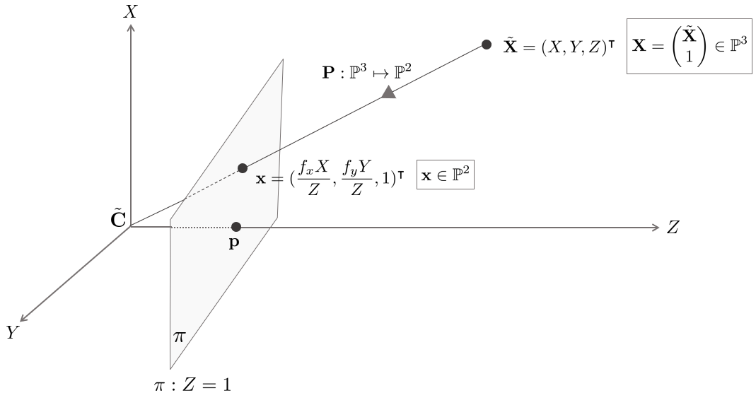
A pinhole camera is when a point $\tilde{\mathbf{X}}$ in $\mathbb{R}^{3}$ space is projected toward a specific center point $\tilde{\mathbf{C}}$ It means a mathematical camera modeling method that expresses an image by forming an image with a point $\mathbf{x}$ on the image plane $\pi \in \mathbb{R}^{2}$ that intersects in the middle. $\tilde{\mathbf{X}}, \tilde{\mathbf{C}}$ means $\mathbf{X}$ represented by Inhomogeneous Coordinate.
\begin{equation}
\begin{aligned}
& \mathbf{X} = \begin{bmatrix} X&Y&Z&1 \end{bmatrix}^{\intercal} \\
& \tilde{\mathbf{X}} = \begin{bmatrix} X&Y&Z \end{bmatrix}^{\intercal} \\
& \mathbf{C} = \begin{bmatrix} c_{x}&c_{y}&c_{z}&1 \end{bmatrix}^{\intercal} \\
& \tilde{\mathbf{C}} = \begin{bmatrix} c_{x}&c_{y}&c_{z}\end{bmatrix}^{\intercal} \\
\end{aligned}
\end{equation}
If we think of an arbitrary $\mathbb{R}^{3}$ space as a camera coordinate system, the origin of the coordinate system is the center point of the camera, $\tilde{\mathbf{C}}$. In general, the image plane $\pi$ is positioned perpendicular to the $Z$ axis. At this time, the $Z$ axis is called the Principal Axis, and the point where the image plane and the Principal Axis meet is called the Principal Point $\mathbf{p}$.
Given a point $\tilde{\mathbf{X}} = \begin{bmatrix} X&Y&Z \end{bmatrix}^{\intercal}$ in 3D space and looking at only the $YZ$ plane, the focal length on the $Y$ axis, which is the distance between the image plane $\pi$ and the camera center point $\tilde{\mathbf{C}}$ ( focal length) $f_{y}$ can be calculated.
\begin{equation}
\begin{aligned}
f_{y}\frac{Y}{Z} = y
\end{aligned}
\end{equation}
Looking at the image plane from the $XZ$ plane, we can calculate $f_{x}$ similarly.
\begin{equation}
\begin{aligned}
f_{x}\frac{X}{Z} = x
\end{aligned}
\end{equation}
Accordingly, the pinhole camera matrix $\mathbf{P}$ can be seen as a linear mapping projecting the point $\tilde{\mathbf{X}} = \begin{pmatrix} X&Y&Z \end{pmatrix}^{\intercal} \in \mathbb{R}^{3}$ in the world onto the 2D image plane $\pi \in \mathbb{R}^{2}$.
\begin{equation}
\begin{aligned}
\mathbf{P}: (X,\ Y,\ Z)^{\intercal} \ \mapsto \ (f_{x}\frac{X}{Z},\ f_{y}\frac{Y}{Z})^{\intercal}
\end{aligned}
\end{equation}
2.1.2. Central projection using homogeneous coordinates
The pinhole camera matrix $\mathbf{P}$ can be thought of as moving a homogeneous point. In other words, the pinhole camera matrix $\mathbf{P}$ can be viewed as a linear map projecting point $\mathbf{X}=\begin{pmatrix} X&Y&Z&1 \end{pmatrix}^{\intercal}$ in space $\mathbb{P}^{3}$ to point $\mathbf{x}=\begin{pmatrix} fX&fY&Z \end{pmatrix}^{\intercal}$ in $\mathbb{P}^{2}$ space. It is assumed that $f=f_{x}=f_{y}$.
\begin{equation}
\begin{aligned}
\mathbf{P}: \begin{pmatrix} X\\Y\\Z\\1 \end{pmatrix} \mapsto \begin{pmatrix} fX \\ fY \\ Z \end{pmatrix} = \begin{bmatrix} f&&&0 \\ &f&&0 \\ &&1&0 \end{bmatrix}\begin{pmatrix} X\\Y\\Z\\1 \end{pmatrix}
\end{aligned}
\end{equation}
Expressing this in matrix form is:
\begin{equation}
\begin{aligned}
\mathbf{x} = \mathbf{PX}
\end{aligned}
\end{equation}
In this case, $\mathbf{P} = \text{diag}(f,f,1)[\mathbf{I}\ |\ 0 ]_{3\times4}$.
2.1.3. Principal point offset

In general, the Principal Point $\mathbf{p}$ is not the origin of the image plane $\pi$. Therefore, in order for the linear mapping through the pinhole camera matrix to properly correspond to the image plane $\pi$, Printcipal Point $\mathbf{p}=\begin{pmatrix} p_{x} & p_{y} \end{pmatrix} ^{\intercal}$ needs to be calibrated
\begin{equation}
\begin{aligned}
\begin{pmatrix} X&Y&Z \end{pmatrix}^{\intercal} \mapsto \begin{pmatrix} fX/Z + p_{x} & fY/Z+p_{y} \end{pmatrix}^{\intercal}
\end{aligned}
\end{equation}
Expressing this at once through the camera matrix $\mathbf{P}$ is:
\begin{equation}
\begin{aligned}
\mathbf{P}: \begin{pmatrix} X\\Y\\Z\\1 \end{pmatrix} \mapsto \begin{pmatrix} fX+Zp_{x} \\ fY+Zp_{y} \\ Z \end{pmatrix} = \begin{bmatrix} f&&p_{x}&0 \\ &f&p_{y}&0 \\ &&1&0 \end{bmatrix}\begin{pmatrix} X\\Y\\Z\\1 \end{pmatrix}
\end{aligned}
\end{equation}
At this time, the matrix $\begin{bmatrix} f&&p_{x} \\ &f&p_{y} \\ &&1 \end{bmatrix}$ is succinctly expressed as $\mathbf{K}$, which is called an intrinsic parameter matrix or camera calibration matrix.
\begin{equation}
\begin{aligned}
\mathbf{K} = \begin{bmatrix} f&&p_{x} \\ &f&p_{y} \\ &&1 \end{bmatrix}
\end{aligned}
\end{equation}
In conclusion, the following $\mathbf{X} \in \mathbb{P}^{3} \mapsto \mathbf{x} \in \mathbb{P}^{2}$ linear mapping is possible through the camera matrix $\mathbf{P}$ including the principal point offset of the camera.
\begin{equation}
\begin{aligned}
\mathbf{x} = \mathbf{K}[\mathbf{I}\ | \ 0]\mathbf{X}
\end{aligned}
\end{equation}
2.1.4. Camera rotation and translation

In general, the camera coordinate system is not the same as the world coordinate system. When the world coordinate system $\{W\}$ is given in the $\mathbb{R}^{3}$ space, the camera coordinate system $\{C\}$, which is positioned $\mathbf{C}=\begin{pmatrix} c_{x}&c_{y}&c_{z}&1 \end{pmatrix}^{\intercal}$ away from it and rotated by $\mathbf{R}$, is The formula for converting a point $\tilde{\mathbf{X}}$ in the world viewed from the world coordinate system $\{W\}$ to a point $\tilde{\mathbf{X}}_{\mathbf{C}}$ on the camera coordinate system $\{C\}$ is as follows.
\begin{equation}
\begin{aligned}
\tilde{\mathbf{X}}_{\mathbf{C}} = \mathbf{R}(\tilde{\mathbf{X}}-\tilde{\mathbf{C}})
\end{aligned}
\end{equation}
When $\mathbf{X}_{\mathbf{C}}$ represented by Homogeneous Coordinate is projected onto the image plane $\pi$, we get:
\begin{equation}
\begin{aligned}
\mathbf{x} = \mathbf{P}\mathbf{X}_{\mathbf{C}} = \mathbf{K}[\mathbf{I}\ | \ 0]\mathbf{X}_{\mathbf{C}}
\end{aligned}
\end{equation}
The detailed expression of $\mathbf{X}_{\mathbf{C}}$ is as follows:
\begin{equation}
\begin{aligned}
\mathbf{X}_{\mathbf{C}} & = \mathbf{R} \begin{bmatrix} 1&&&-c_{x} \\&1&&-c_{y} \\ &&1&-c_{z} \end{bmatrix} \begin{bmatrix} X\\Y\\Z\\1 \end{bmatrix} \\
& = \begin{bmatrix} \mathbf{R} & -\mathbf{R}\tilde{\mathbf{C}} \\ 0 & 1 \end{bmatrix}\begin{bmatrix} X\\Y\\Z\\1 \end{bmatrix} \quad \text{in homogenous coord}
\end{aligned}
\end{equation}
$\mathbf{x} = \mathbf{K}[\mathbf{I}\ | After substituting \ 0]\mathbf{X}_{\mathbf{C}}$ into the formula, it is as follows
\begin{equation}
\begin{aligned}
\mathbf{x} & = \mathbf{K} [\mathbf{I} \ | \ 0 ]\mathbf{X}_{\mathbf{C}}\\
& = \mathbf{K}[\mathbf{I} \ | \ 0]\begin{bmatrix} \mathbf{R} & -\mathbf{R}\tilde{\mathbf{C}} \\ 0 & 1 \end{bmatrix}\begin{bmatrix} X\\Y\\Z\\1 \end{bmatrix} \\
& = \mathbf{K} [\mathbf{R} \ | \ -\mathbf{R}\tilde{\mathbf{C}}]\mathbf{X} \\
& = \mathbf{KR}[\mathbf{I} \ | \ -\tilde{\mathbf{C}}]\mathbf{X}
\end{aligned}
\end{equation}
In general, a method of expressing $\tilde{\mathbf{X}}_{\mathbf{C}}$ based on the world coordinate system, such as $\tilde{\mathbf{X}}_{\mathbf{C}}=\mathbf{R}\tilde{\mathbf{X}} + \mathbf{t}$, is also frequently used. The camera matrix $\mathbf{P}$ is
\begin{equation}
\begin{aligned}
\mathbf{P} = \mathbf{K}[\mathbf{R} \ | \ \mathbf{t}]
\end{aligned}
\end{equation}
The relationship $\mathbf{t} = -\mathbf{R}\tilde{\mathbf{C}}$ is established.
2.1.5. CCD cameras
A CCD camera, one of the most common modern cameras, records image coordinates as the number of pixels. Therefore, when the image coordinates are given in mm, such as $(x,y) [mm]$, it is expressed as $(m_{x}x, \ m_{y}y)$ in the CCD camera. At this time, $m_{x}, m_{y}$ means the number of pixels in the x-axis or y-axis direction within the size of 1 $mm^{2}$. Therefore, when a general camera calibration matrix $\mathbf{K}$ given in mm is given, the following conversion must be performed to convert it to the coordinate system of the CCD camera.
\begin{equation}
\begin{aligned}
\begin{pmatrix} m_{x}&& \\ &m_{y}& \\ &&1 \end{pmatrix} \mathbf{K} = \begin{pmatrix} m_{x}&& \\ &m_{y}& \\ &&1 \end{pmatrix} \begin{pmatrix} f&&p_{x} \\ &f&p_{y} \\ && 1 \end{pmatrix} = \begin{pmatrix} fm_{x} && p_{x}m_{x} \\ &fm_{y} & p_{y}m_{y} \\ 0&0&1 \end{pmatrix}
\end{aligned}
\end{equation}
2.1.6. Finite projective camera
When the camera matrix is given as $\mathbf{P}=\mathbf{K}[\mathbf{R} \ | \ \mathbf{t}]$, this is expressed again as follows
\begin{equation}
\begin{aligned}
\mathbf{P} = \mathbf{KR} [ \mathbf{I} \ | \ -\tilde{\mathbf{C}}] \quad \text{where, } \mathbf{t} = -\mathbf{R}\tilde{\mathbf{C}}
\end{aligned}
\end{equation}
The corresponding camera matrix is called a Finite Projective camera, and $\mathbf{KR}$ must be a non-singular matrix. Given a random non-singular matrix $\mathbf{M} \in \mathbb{R}^{3\times 3}$, the upper triangular matrix $\mathbf{K}$ and the orthogonal matrix $\mathbf{ Since it can be decomposed by R}$, therefore, the set of camera matrices is a set of $\mathbf{P} \in \mathbb{R}^{3\times 4}$-sized matrices, and the left $3\times3$ part of $\mathbf{P}$ is a set that is non-singular.
\begin{equation}
\begin{aligned}
\{\text{set of camera matrix}\} = \{ \mathbf{P} = [\mathbf{M} \ | \ \mathbf{t}] \ | \ \mathbf{M} \text{ is non-singular } 3\times 3 \text{ matrix.}, \mathbf{t} \in \mathbb{R}^{3} \}
\end{aligned}
\end{equation}
2.1.7. General projective cameras
Unlike the previously described finite projective camera, the general projective camera does not require that the $\mathbf{M} \in \mathbb{R}^{3\times 3}$ matrix be non-singular in $\mathbf{P} = [\mathbf{M} \ | \ \mathbf{t}]$, and it means a camera matrix with rank 3 of $\mathbf{P}$.
2.2. The projective camera
2.2.1. Camera anatomy
2.2.2. Camera center
When an arbitrary finite projective camera matrix $\mathbf{P} = \mathbf{KR}[\mathbf{I} \ | \ -\tilde{\mathbf{C}}]$ is given, the following equation holds.
\begin{equation}
\begin{aligned}
\mathbf{PC} = \mathbf{KR}(\mathbf{C}-\mathbf{C}) = \mathbf{0}
\end{aligned}
\end{equation}
$\mathbf{C} \in \mathbb{R}^{4}$ means the center point of the camera or the position of the camera on the world coordinate system, and the camera center point can be obtained by obtaining the null space vector of the rank 3 camera matrix $\mathbf{P} \in \mathbb{R}^{3\times 4}$. Given the camera matrix $\mathbf{P}=\mathbf{KR}[\mathbf{I} \ | \ -\tilde{\mathbf{C}}]$ and when $\mathbf{PC} = \mathbf{0}$ holds, let's say that the point $\mathbf{X}(\lambda)$ on the world is given as follows.
\begin{equation}
\begin{aligned}
\mathbf{X}(\lambda) = \lambda\mathbf{A} + (1-\lambda)\mathbf{C}
\end{aligned}
\end{equation}
This means a line connecting $\mathbf{A}$ and $\mathbf{C}$, and when $\mathbf{X}(\lambda)$ is projected onto the camera, the following equation is obtained
\begin{equation}
\begin{aligned}
\mathbf{x} = \mathbf{PX}(\lambda) = \lambda\mathbf{P}\mathbf{A} + (1-\lambda)\mathbf{PC} = \lambda \mathbf{PA}
\end{aligned}
\end{equation}
In other words, it means that the line connecting points $\mathbf{A}$ and $\mathbf{C}$ on the world becomes a point $\mathbf{x}=\mathbf{\lambda}\mathbf{PA}$ on the image plane regardless of the $\mathbf{C}$ value, which means the property of the center point of the camera. Even in a general general projective camera, the null space vector of $\mathbf{P}$ becomes the camera's center point $\mathbf{C}$.
2.2.3. Column vectors

If the camera matrix $\mathbf{P}$ is expressed as a column vector, it is as follows.
\begin{equation}
\begin{aligned}
& \mathbf{P} = \begin{bmatrix} \mathbf{p}_{1,col} & \mathbf{p}_{2,col} & \mathbf{p}_{3,col} & \mathbf{p}_{4,col} \end{bmatrix}\\
& \text{where, } \mathbf{p}_{i,col} \in \mathbb{R}^{3\times1}, \ i=1,\cdots,4
\end{aligned}
\end{equation}
Among them, $\mathbf{p}_{i,col}, \ i=1,2,3$ means the position of the vanishing points of the $X, Y, Z$ axes, each located on the infinity plane $\pi_{\infty}$. And $\mathbf{p}_{4,col} = \mathbf{P} \begin{pmatrix} 0&0&0&1 \end{pmatrix}^{\intercal}$ means the origin of the field coordinate system.
2.2.4. Row vectors
If the camera matrix $\mathbf{P}$ is expressed as a row vector, it is as follows.
\begin{equation}
\begin{aligned}
& \mathbf{P} = \begin{bmatrix} \mathbf{p}_{1,row}^{\intercal} \\ \mathbf{p}_{2,row}^{\intercal} \\ \mathbf{p}_{3,row}^{\intercal} \end{bmatrix}\\
& \text{where, } \mathbf{p}_{i,row} \in \mathbb{R}^{4\times1}, \ i=1,2,3
\end{aligned}
\end{equation}
The row vectors $\mathbf{p}_{i,row} \ i=1,2,3$ mean planes parallel to the $X,Y,Z$ axes, respectively, based on the camera coordinate system.
2.2.5. The principal plane

The principal plane $\pi_{pp}$ is the plane that contains the center of the camera and is parallel to the image plane. The principal plane is the same as the $XY$ plane in the camera coordinate system $\{C\}$ and is characterized by $Z=0$. Since a point $\mathbf{X} \in \pi_{pp}$ on the principal plane meets the image plane $\pi$ on the line at infinity, the following equation holds.
\begin{equation}
\begin{aligned}
\mathbf{x} = \mathbf{PX} = \begin{pmatrix} x&y&0 \end{pmatrix}^{\intercal}
\end{aligned}
\end{equation}
Therefore, the necessary and sufficient condition for an arbitrary point $\mathbf{X}$ to be located on the principal plane is $\mathbf{p}_{3,row}^{\intercal}\mathbf{X} = 0$. That is, the third row vector $\mathbf{p}_{3,row}$ of the camera matrix means the principal plane of the camera.
2.2.6. The principal point
The principal point $\mathbf{p}$ is the intersection of the principal axis and the image plane $\pi$. The principal point $\mathbf{p}$ is located on the image plane $\pi$, and the straight line connecting the camera center point $\mathbf{C}$ and the principal point is perpendicular to the image plane.
\begin{equation}
\begin{aligned}
\mathbf{p}-\mathbf{C} \perp \pi
\end{aligned}
\end{equation}
You can also define a main point in the following way. Since the main plane is the third row vector $\mathbf{p}_{3,row}$ of the camera matrix, the following expression holds for a point $\mathbf{X}$ located on the main plane.
\begin{equation}
\begin{aligned}
\mathbf{p}_{3,row}^{\intercal}\mathbf{X} = 0
\end{aligned}
\end{equation}
At this time, $\mathbf{p}_{3,row} = \begin{pmatrix} \pi_{1}&\pi_{2}&\pi_{3}&\pi_{4} \end{pmatrix}^{\intercal}$ means the normal vector of the $\mathbf{p}_{3,row}$ plane in the Dual Projective Space $(\mathbb{P}^{3})^{\vee}$. The intersection of the main plane $\mathbf{p}_{3,row}$ and the plane at infinity $\pi_{\infty}$ becomes the normal vector $\begin{pmatrix} \pi_{1}&\pi_{2}&\pi_{3}&0 \end{pmatrix}^{\intercal}$ existing in the plane at infinity. In conclusion, the point projected onto the image plane becomes the principal point $\mathbf{p}$.
\begin{equation}
\begin{aligned}
\mathbf{p} = \mathbf{P} \begin{pmatrix} \pi_{1}\\\pi_{2}\\\pi_{3}\\0 \end{pmatrix}
\end{aligned}
\end{equation}
The normal vector $\begin{bmatrix} \pi_{1}&\pi_{2}&\pi_{3}&0 \end{bmatrix}^{\intercal}$ that passes through the camera center point $\mathbf{C}$ and exists on the infinity plane is equal to the principal axis, so if the principal axis is projected onto the image plane as shown in the equation below, it becomes the principal point $\mathbf{p}$.
\begin{equation}
\begin{aligned}
\mathbf{P}\bigg( \lambda \begin{pmatrix} \pi_{1}\\\pi_{2}\\\pi_{3}\\0 \end{pmatrix} + (1-\lambda)\mathbf{C} \bigg) = \lambda \mathbf{P}\begin{pmatrix} \pi_{1}\\\pi_{2}\\\pi_{3}\\0 \end{pmatrix} = \mathbf{p}
\end{aligned}
\end{equation}
In conclusion, the principal point $\mathbf{p}$ means the first three terms $\mathbf{p} = (\pi_{1},\pi_{2},\pi_{3})^{\intercal}$ in the third row vector $\mathbf{p}_{3,row} = \begin{bmatrix} \pi_{1}&\pi_{2}&\pi_{3}&p_{4} \end{bmatrix}^{\intercal}$ of the camera matrix $\mathbf{P}$.
2.2.7. The principal axis vector
Given the camera matrix $\mathbf{P} = [\mathbf{M} \ | \ \mathbf{p}_{4,col}]$, the third row vector $\mathbf{m}_{3,row}$ of the matrix $\mathbf{M} \in \mathbb{R}^{3\times 3}$ means the principal point.In this section, the principal point $\mathbf{m}_{3,row}$ is considered equivalent to the direction of the principal axis, which means the $+Z$ direction in the camera coordinate system. However, since the camera matrix $\mathbf{P}$ is uniquely determined up to sign, it is not known which $\mathbf{m}_{3,row}$ or $-\mathbf{m}_{3,row}$ means $+Z$.
At this time, multiplying the determinant of $\mathbf{M}$ in front, like $\mathbf{v} = \det(\mathbf{M})\mathbf{m}_{3,row} = (0,0,1)^{\intercal}$, always means the positive direction. And even if the scale changes to $\mathbf{P} \rightarrow k \mathbf{P}$, it shows the same direction as $\mathbf{v} \rightarrow k^{4}\mathbf{v}$. Even when a general camera matrix $k\mathbf{P} = k\mathbf{KR}[\mathbf{I} \ | \ -\tilde{\mathbf{C}}]$ is given, since it is $\mathbf{M} = k \mathbf{KR}$ and $\det(\mathbf{R}) > 0$, the direction vector $\mathbf{v}=\det(\mathbf{M})\mathbf{m}_{3,rowe}$ of the main axis indicates the same direction. Accordingly, the vector $\mathbf{v}$ means the direction vector of the principal axis.
\begin{equation}
\begin{aligned}
\mathbf{v} = \det(\mathbf{M})\mathbf{m}_{3,row}
\end{aligned}
\end{equation}
2.2.8. Action of a projective camera on points
2.2.9. Forward projection
Forward-projection is generally called projection, and refers to an operation that converts a given point $\mathbf{X}$ on the world into a point $\mathbf{x}$ on the image plane. For any camera matrix $\mathbf{P}$, the following formula holds.
\begin{equation}
\begin{aligned}
\mathbf{x} = \mathbf{PX}
\end{aligned}
\end{equation}
2.2.10. Back-projection of points to rays

Back-projection is the opposite of forward-projection. When a point on the image plane $\mathbf{x}$ is given, it means an operation that transforms it into a straight line in the world. In general, since the depth value of $\mathbf{x}$ is not known, it is not immediately converted to a point $\mathbf{X}$ in the world. Since any camera matrix $\mathbf{P}$ has a rank of 3, a Right Pseudo Inverse $\mathbf{P}^{\dagger}$ exists.
\begin{equation}
\begin{aligned}
\mathbf{P}^{\dagger} = \mathbf{P}^{\intercal}(\mathbf{PP}^{\intercal})^{-1}
\end{aligned}
\end{equation}
At this time, $\mathbf{PP}^{\dagger} = \mathbf{PP}^{\intercal}(\mathbf{PP}^{\intercal})^{-1} = \mathbf{I}$ is established. Since the back-projected line $\mathbf{P}^{\dagger}\mathbf{x}$ passes through the center point $\mathbf{C}$ of the camera, it can be expressed as follows.
\begin{equation}
\begin{aligned}
\mathbf{X}(\lambda) = \mathbf{P}^{\dagger}\mathbf{x} + \lambda \mathbf{C}
\end{aligned}
\end{equation}
If you project the back-projected straight line, it becomes $\mathbf{P}\mathbf{X}(\lambda) = \mathbf{PP}^{\dagger}\mathbf{x} + \lambda \mathbf{PC} = \mathbf{x}$.
In the case of finite projective cameras, back-projection can be expressed in a different way. Given an arbitrary finite projective camera matrix $\mathbf{P}=[\mathbf{M} \ | \ \mathbf{p}_{4,col}]$, the center point of the camera can be expressed as $\tilde{\mathbf{C}}=-\mathbf{M}^{-1}\mathbf{p}_{4,col}$. At this time, the straight line back-projected from a point $\mathbf{x}$ on the image plane meets the infinity plane $\pi_{\infty}$ at $\mathbf{D}=((\mathbf{M}^{-1}\mathbf{x})^{\intercal},0)$, so the back-projection straight line can be expressed as follows.
\begin{equation}
\begin{aligned}
\mathbf{X}(\mu) = \mu \begin{pmatrix} \mathbf{M}^{-1}\mathbf{x}\\0 \end{pmatrix} + \begin{pmatrix} -\mathbf{M}^{-1}\mathbf{p}_{4,col} \\ 1 \end{pmatrix} = \begin{pmatrix} \mathbf{M}^{-1}(\mu \mathbf{x} - \mathbf{p}_{4,col}) \\ 1 \end{pmatrix}
\end{aligned}
\end{equation}
2.2.11. Depth of points
Given a General Projective camera $\mathbf{P}$ and a point $\mathbf{X}=\begin{pmatrix} X&Y&Z&1 \end{pmatrix}^{\intercal}$ in the world, if it is projected onto the image plane, a single point $\mathbf{x}$ can be obtained as shown below.
\begin{equation}
\begin{aligned}
\mathbf{x} = \mathbf{P}\begin{pmatrix} X\\Y\\Z\\1 \end{pmatrix} = \begin{pmatrix} x\\y\\w \end{pmatrix}
\end{aligned}
\end{equation}
2.2.12. Result 6.1

The depth of a point $\mathbf{X}$ in the world for a camera matrix $\mathbf{P}$ is:
\begin{equation}
\begin{aligned}
\text{depth}(\mathbf{X}; \mathbf{P}) = \frac{\text{sign}(\det(M))w}{\|\mathbf{m}_{3,row} \|}
\end{aligned}
\end{equation}
$\mathbf{m}_{3,row} \in \mathbb{R}^{3\times 3}$ is the third row vector of matrix $\mathbf{M}$.
2.2.13. Proof
Since the row vector $\mathbf{m}_{3,row}$ means the direction of the main axis, the value obtained by projecting the point $\tilde{\mathbf{X}}$ in the world to $\mathbf{m}_{3,row}$ means the depth on the $Z$ axis. The projection on the main axis is:
\begin{equation}
\begin{aligned}
\text{depth} = \frac{(\tilde{\mathbf{X}}-\tilde{\mathbf{C})}\mathbf{m}_{3.row}}{\| \mathbf{m}_{3,row} \|}
\end{aligned}
\end{equation}
For Finite Projective cameras, $\mathbf{m}_{3,row} = \mathbf{r}_{3,row} = 1$. Since the depth value is $w$, which is the third row of $\mathbf{x} = \mathbf{PX}$, it can be obtained as follows.
\begin{equation}
\begin{aligned}
w & = (\mathbf{PX})_{3,row} \\
& = (\mathbf{P}(\mathbf{X}-\mathbf{C}))_{3,row} \\
& = (\tilde{\mathbf{X}}-\tilde{\mathbf{C}})\mathbf{m}_{3,row} \\
\end{aligned}
\end{equation}
In conclusion, since the depth value can be located behind the camera according to the sign of $\det(\mathbf{M})$, taking this into account, the expression is as follows.
\begin{equation}
\begin{aligned}
\text{depth}(\mathbf{X}; \mathbf{P}) = \frac{\text{sign}(\det(M))w}{\|\mathbf{m}_{3,row} \|}
\end{aligned}
\end{equation}
2.3. Cameras at infinity

If the center point $\mathbf{C}$ of any General Projective camera exists on the infinity plane $\pi_{\infty}$, it is called a camera at infinity.
\begin{equation}
\begin{aligned}
\mathbf{C} =(\ast,\ \ast,\ \ast, 0)^{\intercal} \in \pi_{\infty}
\end{aligned}
\end{equation}
An equivalent case is when the matrix $\mathbf{M}$ is singular when the camera matrix $\mathbf{P}=[\mathbf{M} \ | \ \mathbf{p}_{4,col}]$ is given. Infinity cameras are classified into affine cameras and non-affine cameras.
2.3.1. Definition 6.3

Affine camera $\mathbf{P}_{A}$ means a camera that becomes the same infinite plane when projected onto an infinity plane.
\begin{equation}
\begin{aligned}
\mathbf{P}_{A}(\pi_{\infty}) = \pi_\infty
\end{aligned}
\end{equation}
이 때, $\mathbf{P}_{A} = \begin{bmatrix} \ast&\ast&\ast&\ast \\ \ast&\ast&\ast&\ast \\ 0&0&0&\ast \end{bmatrix}$ 꼴이다.
2.3.2. Affine cameras

Let's say there is a finite projective camera matrix $\mathbf{P}=\mathbf{KR}[\mathbf{I} \ | \ 0]$ and there are objects in the world. At this time, if you zoom in on an object and move the camera in the opposite direction of the main axis at the same time, the Vertigo Effect occurs. The Vertigo Effect was named after the first use of the technique in Hitchcock's movie Vertigo.
In order to understand this mathematically, if we think about the depth value of an object in the world again, when the center point $\tilde{\mathbf{C}}$ of the camera is given and the point $\tilde{\mathbf{X}}$ in the world is given, the depth value $d$ is as follows.
\begin{equation}
\begin{aligned}
d = -(\tilde{\mathbf{X}}-\tilde{\mathbf{C}})\mathbf{r}_{3,row}
\end{aligned}
\end{equation}
At this time, $\mathbf{r}_{3,row}$ is the third row vector of the rotation matrix $\mathbf{R}$ and means the principal axis. Next, if the distance between the camera center point and the world origin is $d_{0}$, it corresponds to the case of $\tilde{\mathbf{X}}=0$ in the above formula, so the following formula holds.
\begin{equation}
\begin{aligned}
d_{0} = - \tilde{\mathbf{C}}\mathbf{r}_{3,row}
\end{aligned}
\end{equation}
If you move the camera in the opposite direction of the main axis, the center point of the camera $\tilde{\mathbf{C}}$ is
\begin{equation}
\begin{aligned}
\tilde{\mathbf{C}} - t\cdot \mathbf{r}_{3,row}
\end{aligned}
\end{equation}
$t$ stands for time. When the camera moves backwards, the camera matrix over time is as follows:
\begin{equation}
\begin{aligned}
\mathbf{P}_{t} & = \mathbf{KR}[\mathbf{I} \ | \ -(\tilde{\mathbf{C}}-t\cdot \mathbf{r}_{3,row})] \\
& = \mathbf{K}
\begin{bmatrix}
& & & -\tilde{\mathbf{C}}\mathbf{r}_{1,row} \\
& \mathbf{R} & & -\tilde{\mathbf{C}}\mathbf{r}_{2,row} \\
& & & t -\tilde{\mathbf{C}}\mathbf{r}_{3,row} \\
\end{bmatrix} \\
& = \mathbf{K}
\begin{bmatrix}
& & & -\tilde{\mathbf{C}}\mathbf{r}_{1,row} \\
& \mathbf{R} & & -\tilde{\mathbf{C}}\mathbf{r}_{2,row} \\
& & & d_{0} + t \\
\end{bmatrix} \\
\end{aligned}
\end{equation}
Therefore, when the camera is moved in the opposite direction of the main axis, $\mathbf{P}_{t}$ becomes a form in which $d_{0} + t$ is added only to the $(3,4)$ term. The $d_{0} + t = d_{t}$ is as follows
\begin{equation}
\begin{aligned}
\mathbf{P}_{t} = \mathbf{K} \begin{bmatrix} -&-&-&- \\ -&\text{no change}&-&- \\ -&-&-&d_{t} \end{bmatrix}
\end{aligned}
\end{equation}
Next, let's zoom in on the camera. The mathematical expression of Zoom In is the same as increasing the size of the focal length $f$.
\begin{equation}
\begin{aligned}
\text{Zoom In}: f \rightarrow kf \quad ^{\forall}k > 0
\end{aligned}
\end{equation}
Expressing Zoom In as a matrix is as follows.\begin{equation}
\begin{aligned}
\mathbf{P} \rightarrow \begin{bmatrix} k&& \\ &k& \\ &&1 \end{bmatrix}\mathbf{P}
\end{aligned}
\end{equation}
At this time, if you zoom in by multiplying the focal length $k$ while moving the camera in the direction of the main axis, you can realize the Vertigo Effect that keeps the depth of the object unchanged. At this time, the appropriate Zoom In value $k$ is as follows
\begin{equation}
\begin{aligned}
k = d_{t}/d_{0}
\end{aligned}
\end{equation}
After all, the time-dependent camera matrix $\mathbf{P}_{t}$ is
\begin{equation}
\begin{aligned}
\begin{bmatrix} d_{t}/d_{0}&& \\ &d_{t}/d_{0}& \\ &&1 \end{bmatrix} \mathbf{P}_{t} & = \mathbf{K} \begin{bmatrix} d_{t}/d_{0}&& \\ &d_{t}/d_{0}& \\ &&1 \end{bmatrix} \begin{bmatrix} &&&\ast \\ &\mathbf{R}&&\ast \\ &&&d_{t} \end{bmatrix} \\
& = \frac{1}{k}\mathbf{K} \begin{bmatrix} 1&& \\ &1& \\ &&d_{0}/d_{t} \end{bmatrix} \begin{bmatrix} &&&\ast \\ &\mathbf{R}&&\ast \\ &&&d_{t} \end{bmatrix} \\
& = \frac{1}{k}\mathbf{K} \begin{bmatrix} -&-&-&- \\ -&\text{no change}&-&- \\ &d_{0}/d_{t} \cdot \mathbf{r}_{3,row}&&d_{0} \end{bmatrix} \\
\end{aligned}
\end{equation}
Since $\frac{1}{k}$ is a scale value, it can be omitted. Assuming that time elapses infinitely, the following equation becomes
\begin{equation}
\begin{aligned}
\mathbf{P}_{\infty} = \lim_{t\rightarrow \infty} \mathbf{P}_{t} = \mathbf{K} \begin{bmatrix} \mathbf{r}_{1,row}^{\intercal} & -\mathbf{r}_{1,row}^{\intercal}\tilde{\mathbf{C}} \\ \mathbf{r}_{2,row}^{\intercal} & -\mathbf{r}_{2,row}^{\intercal}\tilde{\mathbf{C}} \\ \mathbf{0}^{\intercal} & d_{0} \end{bmatrix}
\end{aligned}
\end{equation}
In the above equation, since the three values in the third row of $\mathbf{P}$ are $\mathbf{0}^{\intercal}$, this is an Affine camera.
2.3.3. Error in employing and affine camera
This section explains how big the difference is between taking pictures of the same object with a General Projective camera and an Affine camera. A general projective camera is denoted by $\mathbf{P}_{0}$, an affine camera is denoted by $\mathbf{P}_{\infty}$, and the change of the camera matrix according to time $t$ is denoted by $\mathbf{P}_{t}$.
When a plane $\pi$ including the origin of the world coordinate system and perpendicular to the image plane of camera $\mathbf{P}_{t}$ is given, performing the Vertigo Effect(zoom in + backward moving) described above, the points located at $\pi$ on the image obtained by $\mathbf{P}_{t}$ are constant with respect to $t$.
To prove this, when a point $\mathbf{X} \in \pi$ is given on the plane $\pi$, since $\pi$ includes the origin of the world coordinate system, it can be expressed as follows
\begin{equation}
\begin{aligned}
& \mathbf{X} = \begin{pmatrix} \alpha \mathbf{r}_{1,row} + \mathbf{\beta}\mathbf{r}_{2,row} \\ 1 \end{pmatrix} \in \mathbb{R}^{4}
\end{aligned}
\end{equation}
Projecting this through $\mathbf{P}_{t}$ gives
\begin{equation}
\begin{aligned}
\mathbf{P}_{t}\mathbf{X} & = \mathbf{K} \begin{bmatrix} \mathbf{r}_{1,row}^{\intercal} & -\mathbf{r}_{1,row}^{\intercal}\tilde{\mathbf{C}} \\ \mathbf{r}_{2,row}^{\intercal} & -\mathbf{r}_{2,row}^{\intercal}\tilde{\mathbf{C}} \\ d_{0}/d_{t} \cdot \mathbf{r}_{3,row} & d_{0} \end{bmatrix} \begin{bmatrix} \alpha \mathbf{r}_{1,row} + \beta \mathbf{r}_{2,row} \\ 1 \end{bmatrix} \\
& = \begin{bmatrix} * \\ * \\ d_{0} \end{bmatrix} \\
& \because \mathbf{r}_{1,row}\cdot \mathbf{r}_{3,row} = \mathbf{r}_{2,row}\cdot \mathbf{r}_{3,row}= 0 \
\end{aligned}
\end{equation}
Therefore, since the depth of the point $\mathbf{X}$ on the plane $\pi$ containing the origin of the world coordinate system is $d_{0}$ and is always constant, performing the Vertigo Effect appears to have a constant size regardless of time $t$. That is, both $\mathbf{X}$ in the General Projective camera and the Affine camera are converted to points on the same image.
\begin{equation}
\begin{aligned}
\mathbf{P}_{0}\mathbf{X} = \mathbf{P}_{t}\mathbf{X} = \mathbf{P}_{\infty}\mathbf{X}
\end{aligned}
\end{equation}
If two cameras take a point $\mathbf{X}^{\prime}$ in the world that is a distance of $\Delta$ from the plane $\pi$, not a point on the plane $\pi$ perpendicular to the image plane passing through the origin of the world coordinate system, it becomes $\mathbf{P}_{0}\mathbf{X}^{\prime} \neq \mathbf{P}_{\infty}\mathbf{X}^{\prime}$. $\mathbf{X}^{\prime}$ can be expressed as:
\begin{equation}
\begin{aligned}
\mathbf{X}^{\prime} = \begin{pmatrix} \alpha \mathbf{r}_{1,row} + \beta \mathbf{r}_{2,row} + \Delta \mathbf{r}_{3,row} \\ 1 \end{pmatrix}
\end{aligned}
\end{equation}
In this case, $\mathbf{r}_{3,row}$ means the principal axis of the camera. Projecting $\mathbf{X}^{\prime}$ onto both cameras gives:
\begin{equation}
\begin{aligned}
\mathbf{x}_{\text{proj}} & = \mathbf{P}_{0}\mathbf{X}^{\prime} = \mathbf{K}\begin{pmatrix} \tilde{x}\\\tilde{y}\\\tilde{z}_{\text{proj}} \end{pmatrix}
& = \mathbf{K}\begin{pmatrix}
\alpha - \mathbf{r}_{1,row}^{\intercal}\tilde{\mathbf{C}} \\
\beta - \mathbf{r}_{2,row}^{\intercal}\tilde{\mathbf{C}} \\
d_{0} + \Delta
\end{pmatrix}
\end{aligned}
\end{equation}
\begin{equation}
\begin{aligned}
\mathbf{x}_{\text{affine}} & = \mathbf{P}_{\infty}\mathbf{X}^{\prime} = \mathbf{K}\begin{pmatrix} \tilde{x}\\\tilde{y}\\\tilde{z}_{\text{affine}} \end{pmatrix}
& = \mathbf{K}\begin{pmatrix}
\alpha - \mathbf{r}_{1,row}^{\intercal}\tilde{\mathbf{C}} \\
\beta - \mathbf{r}_{2,row}^{\intercal}\tilde{\mathbf{C}} \\
d_{0}
\end{pmatrix}
\end{aligned}
\end{equation}
$\tilde{z}_{\text{proj}}$ can be obtained as follows.
\begin{equation}
\begin{aligned}
\tilde{z}_{\text{proj}} & = [\mathbf{r}_{3,row} | -\mathbf{r}_{3,row}\tilde{\mathbf{C}}]\mathbf{X}^{\prime} \\
& = [\mathbf{r}_{3,row} | -\mathbf{r}_{3,row}\tilde{\mathbf{C}}]\begin{pmatrix} \alpha \mathbf{r}_{1,row} + \beta \mathbf{r}_{2,row} + \Delta \mathbf{r}_{3,row} \\ 1 \end{pmatrix} \\
& = -\mathbf{r}_{3,row}\tilde{\mathbf{C}} + \Delta \\
& = d_{0} + \Delta
\end{aligned}
\end{equation}
The camera calibration matrix $\mathbf{K}$ can be expressed as follows.
\begin{equation}
\begin{aligned}
\mathbf{K} = \begin{bmatrix} \mathbf{K}_{2\times 2} & \tilde{\mathbf{x}}_{0} \\ \tilde{0}^{\intercal} & 1 \end{bmatrix}
\end{aligned}
\end{equation}
At this time, $\mathbf{K}_{2\times 2}$ means an upper-triangular matrix with a size of $2\times 2$, and $\tilde{\mathbf{x}}_{0} = \begin{pmatrix} x_{0} & y_{0} \end{pmatrix}^{\intercal}$ means the origin of the image plane. Taking this into account, the above formulas are rearranged as follows:
\begin{equation}
\begin{aligned}
& \mathbf{x}_{\text{proj}} = \begin{pmatrix} \mathbf{K}_{2\times 2}\tilde{\mathbf{x}} + (d_{0}+\Delta)\tilde{\mathbf{x}}_{0} \\ d_{0} + \Delta \end{pmatrix} \\
& \mathbf{x}_{\text{affine}} = \begin{pmatrix} \mathbf{K}_{2\times 2}\tilde{\mathbf{x}} + d_{0}\tilde{\mathbf{x}}_{0} \\ d_{0} \end{pmatrix} \\
\end{aligned}
\end{equation}
In this case, $\tilde{\mathbf{x}} = \begin{pmatrix} \tilde{x} & \tilde{y} \end{pmatrix}^{\intercal}$. When calculating the Inhomogeneous coordinates of the two points $\mathbf{x}_{\text{proj}}$ and $\mathbf{x}_{\text{affine}}$, it is the value divided by the last term, so the following equation holds.
\begin{equation}
\begin{aligned}
& \tilde{\mathbf{x}}_{\text{proj}} = \tilde{\mathbf{x}}_{0} + \mathbf{K}_{2\times 2}\tilde{\mathbf{x}}/(d_{0}+\Delta) \\
& \tilde{\mathbf{x}}_{\text{affine}} = \tilde{\mathbf{x}}_{0} + \mathbf{K}_{2\times 2}\tilde{\mathbf{x}}/d_{0} \\
\end{aligned}
\end{equation}
In conclusion, the difference between the two points projected by the general projective camera and the affine camera is as follows.
\begin{equation}
\begin{aligned}
\tilde{\mathbf{x}}_{\text{affine}} - \tilde{\mathbf{x}}_{0} = \frac{d_{0}+\Delta}{d_{0}} (\tilde{\mathbf{x}}_{\text{proj}} - \tilde{\mathbf{x}}_{0})
\end{aligned}
\end{equation}
The above formula is called the Discrepancy Equation, and in the case of $\Delta=0$, it means that an object photographed by two cameras is projected as a point on the same image if it is a point on a plane $\pi$ that is perpendicular to the image plane and includes the origin of the world coordinate system. If you watch the movie Vertigo or Jaws, you can see this phenomenon. You can see that the surrounding environment is zoomed out while the main character's face does not change.
3. Computation of the Camera Matrix $\mathbf{P}$
This section describes how to numerically obtain the camera matrix $\mathbf{P}$ using several corresponding pairs $(\mathbf{x}_{i}, \mathbf{X}_{i})$ of points $\mathbf{X}_{i}$ in $\mathbb{P}^{3}$ space and points $\mathbf{x}_{i}$ in $\mathbb{P}^{2}$ space. This method is generally called Resectioning or Calibration.
3.1. Basic equations
Given a pair of correspondence points $(\mathbf{x}_{i}, \mathbf{X}_{i})$, the correspondence between the two points is as follows.
\begin{equation}
\begin{aligned}
\mathbf{x}_{i} = \mathbf{PX}_{i}
\end{aligned}
\end{equation}
At this time, $\mathbf{PX}_{i}$ can be expressed using a row vector as follows:
\begin{equation}
\begin{aligned}
\mathbf{PX}_{i} & = \begin{bmatrix} \mathbf{p}_{1,row}^{\intercal} \\ \mathbf{p}_{2,row}^{\intercal} \\ \mathbf{p}_{3,row}^{\intercal} \end{bmatrix}\mathbf{X}_{i}
& = \begin{bmatrix}
\mathbf{p}_{1,row}^{\intercal}\mathbf{X}_{i} \\
\mathbf{p}_{2,row}^{\intercal}\mathbf{X}_{i} \\
\mathbf{p}_{3,row}^{\intercal}\mathbf{X}_{i}
\end{bmatrix}
\end{aligned}
\end{equation}
In this case, it means a vector of $\mathbf{p}_{i,row} \in \mathbb{R}^{4\times 1}$. If $\mathbf{x} = \begin{pmatrix} x&y&w \end{pmatrix}^{\intercal}$ is $\mathbf{x}_{i} \times \mathbf{PX}_{i}=0$, it is as follows
\begin{equation}
\begin{aligned}
\mathbf{x}_{i} \times \mathbf{PX}_{i} =
\begin{pmatrix}
y_{i}\cdot\mathbf{p}_{2,row}^{\intercal}\mathbf{X}_{i} - w_{i}\cdot\mathbf{p}_{3,row}\mathbf{X}_{i} \\
w_{i}\cdot\mathbf{p}_{1,row}^{\intercal}\mathbf{X}_{i} - x_{i}\cdot\mathbf{p}_{3,row}\mathbf{X}_{i} \\
x_{i}\cdot\mathbf{p}_{2,row}^{\intercal}\mathbf{X}_{i} - y_{i}\cdot\mathbf{p}_{1,row}\mathbf{X}_{i} \\
\end{pmatrix} = 0
\end{aligned}
\end{equation}
If we arrange this in the form of $\mathbf{Ap} = 0$, we get:
\begin{equation}
\begin{aligned}
\begin{bmatrix}
\mathbf{0}^{\intercal} & -w_{i}\mathbf{X}_{i}^{\intercal} & y_{i}\mathbf{X}_{i}^{\intercal} \\
w_{i}\mathbf{X}_{i}^{\intercal} & \mathbf{0}^{\intercal} & -x_{i}\mathbf{X}_{i}^{\intercal} \\
-y_{i}\mathbf{X}_{i}^{\intercal} & x_{i}\mathbf{X}_{i}^{\intercal} & \mathbf{0}^{\intercal} \\
\end{bmatrix}
\begin{pmatrix} \mathbf{p}_{1,row} \\ \mathbf{p}_{2,row} \\ \mathbf{p}_{3,row} \end{pmatrix} = 0
\end{aligned}
\end{equation}
Since the last row of the matrix on the left is linearly dependent, expressing only the first and second rows is as follows:
\begin{equation}
\begin{aligned}
\underbrace{\begin{bmatrix}
\mathbf{0}^{\intercal} & -w_{i}\mathbf{X}_{i}^{\intercal} & y_{i}\mathbf{X}_{i}^{\intercal} \\
w_{i}\mathbf{X}_{i}^{\intercal} & \mathbf{0}^{\intercal} & -x_{i}\mathbf{X}_{i}^{\intercal} \\
\end{bmatrix}}_{\mathbf{A}}
\begin{pmatrix} \mathbf{p}_{1,row} \\ \mathbf{p}_{2,row} \\ \mathbf{p}_{3,row} \end{pmatrix} = 0
\end{aligned}
\end{equation}
At this time, the matrix $\mathbf{A}$ is of size $\mathbb{R}^{2n\times 12}$ and the vector $\begin{pmatrix} \mathbf{p}_{1,row} \\ \mathbf{p}_{2,row} \\ \mathbf{p}_{3,row} \end{pmatrix}$ is of size $12\times1$. Since the equation above is of the form $\mathbf{Ap}=0$, the vector $\mathbf{p}$ can be obtained through a method such as singular value decomposition (SVD).
3.1.1. Minimal solution
A total of 11 equations are required to obtain the vector $\mathbf{p} \in \mathbb{R}^{12}$ up to scale. Since two equations are derived using one correspondence point pair $(\mathbf{x}_{i}, \mathbf{X}_{i})$, at least 5.5 correspondence point pairs are required to obtain $\mathbf{p}$. Given 5.5 pairs of correspondence points without noise, the rank of the matrix $\mathbf{A}$ becomes 11, and the null space vector becomes the unique solution vector $\mathbf{p}$.
3.1.2. Over-determined solution
In general, the number of pairs of corresponding points $(\mathbf{x}_{i}, \mathbf{X}_{i})$ can be much higher than 6, and since the data contains noise, the rank of matrix $\mathbf{A}$ is It becomes 12. Therefore, since the null space does not exist, the solution vector $\mathbf{p}$ cannot be obtained. .This $\mathbf{Ap}=0$ linear system is called an over-determined system, and in this case, an approximate solution $\hat{\mathbf{p}}$ that minimizes the magnitude of $\|\mathbf{Ap} \|$ must be obtained for the case of $\|\mathbf{p} \|=1$.
3.1.3. Degenerate configurations
If 5.5 or more pairs of corresponding points $(\mathbf{x}_{i}, \mathbf{X}_{i})$ are not linearly independent of each other, the unique solution vector $\mathbf{p}$ cannot be determined, and These pairs of correspondence points are called Degenerate Configurations. This means that the unique solution vector $\mathbf{p}$ cannot be determined. For a point $\mathbf{X}$ in the world, any other camera matrix $\mathbf{P}^{\prime}$ that satisfies the following equation exists.
\begin{equation}
\begin{aligned}
& ^{\exists}\mathbf{P}^{\prime}, \ \ \mathbf{P} \neq \mathbf{P}^{\prime} \\
& \mathbf{PX}_{i} = \mathbf{P}^{\prime}\mathbf{X}_{i} \quad ^{\forall}i
\end{aligned}
\end{equation}
This is the same as the meaning that $\mathbf{PX} = -\theta \mathbf{P}^{\prime}\mathbf{X}$ also holds for a specific constant $\theta$.
\begin{equation}
\begin{aligned}
\underbrace{(\mathbf{P} + \theta \mathbf{P}^{\prime})}_{\mathbf{P}_{\theta}}\mathbf{X} = 0 \quad \text{for some } \theta
\end{aligned}
\end{equation}
A point $\mathbf{X}$ in the world that satisfies $\mathbf{P}_{\theta}\mathbf{X}=0$ cannot distinguish between $\mathbf{P}$ and $\mathbf{P}^{\prime}$. In this way, if the set of $\mathbf{X}$ transferred to a point on the same image plane by $\mathbf{P}, \mathbf{P}^{\prime}$ is $\mathcal{S}_{\theta}$, it is as follows
\begin{equation}
\begin{aligned}
\mathcal{S}_{\theta} = \{ \mathbf{X} \ | \ \mathbf{P}_{\theta}\mathbf{X}=0 \}
\end{aligned}
\end{equation}
The point $\mathbf{X}$ in the world that satisfies $\mathcal{S}_{\theta}$ is as follows.
- When all $\mathbf{X}_{i}$ are located on Twisted Cubic
- If all $\mathbf{X}_{i}$ exist on the same plane and on a straight line including the camera center point
Twisted Cubic means a curve that exists in $\mathbb{P}^{3}$ space. The set $\mathcal{C}_{\theta}$ composed of Twisted Cubic $\mathbf{C}_{\theta}$ means a set that satisfies the following expression.
\begin{equation}
\begin{aligned}
\mathcal{C}_{\theta} = \{ \mathbf{C}_{\theta} \ | \ \mathbf{P}_{\theta}\mathbf{C}_{\theta}=0 \ \text{ and } \mathbf{P}_{\theta} \text{'s rank is 3} \}
\end{aligned}
\end{equation}
$\mathbf{C}_{\theta}$ appears in the form of a cubic expression, and sometimes it is not Twisted Cubic due to the intermediate root, but it generally means Twisted Cubic.Since it is $\mathbf{P}_{\theta}\mathbf{C}_{\theta}=0$ and the rank of $\mathbf{P}_{\theta}$ is 3, it means that $\mathbf{C}_{\theta}$ is in the row space of $\mathbf{P}_{\theta}$.
\begin{equation}
\begin{aligned}
\mathbf{C}_{\theta} = \text{Row } \mathbf{P}_{\theta}
\end{aligned}
\end{equation}
따라서 $\mathbf{C}_{\theta} = \begin{pmatrix} c_{1}&c_{2}&c_{3}&c_{4} \end{pmatrix}$일 때
\begin{equation}
\begin{aligned}
\det \begin{pmatrix} c_{1}&c_{2}&c_{3}&c_{4} \\ -&-&-&- \\ -&\mathbf{P}_{\theta}&-&- \\ -&-&-&- \end{pmatrix} = 0
\end{aligned}
\end{equation}
When this is expanded, it becomes $\det(2\ 3\ 4)c_{1} -\det(1\ 3\ 4)c_{2} + \det(1\ 2\ 4)c_{3} -\det(1\ 2\ 3)c_{4}=0$. At this time, $\det(a\ b\ c)$ means the sub-determinant (subminor) of the $a,b,c$ row and column of matrix $\mathbf{P}_{\theta}$. By rearranging $\mathbf{C}_{\theta}$ through this, each term is a cubic twisted cubic as follows:
\begin{equation}
\begin{aligned}
\mathbf{C}_{\theta} = (\det(2\ 3\ 4), -\det(1\ 3\ 4), \det(1\ 2\ 4), -\det(1\ 2\ 3))
\end{aligned}
\end{equation}
According to $\mathbf{P}, \mathbf{P}^{\prime}$, all terms in $\mathbf{C}_{\theta}$ can have a common root, and each term's degree is 3 or less. can fall to This case is called Degenerate Configuration of $\mathbf{C}_{\theta}$, and this $\mathbf{C}_{\theta}$ is not Twisted Cubic.
3.1.4. Line correspondences
When a straight line $\mathbf{L}$ in the world is projected with the camera matrix $\mathbf{P}$ to obtain a straight line $\mathbf{l}$ on the image plane, unlike a point, the straight line is $\mathbf{l} \neq \mathbf{PL}$.
\begin{equation}
\begin{aligned}
& \mathbf{x} = \mathbf{PX} \ \text{ but, } \ \mathbf{l} \neq \mathbf{PL} \\
\end{aligned}
\end{equation}
Since the point $\mathbf{x}$ obtained by projecting a point $\mathbf{X}$ on the straight line $\mathbf{L}$ to the camera exists on the straight line $\mathbf{l}$, the following linear equation for vector $\mathbf{p}$ is established.
\begin{equation}
\begin{aligned}
& \mathbf{l}^{\intercal}\mathbf{x} = \mathbf{l}^{\intercal}\mathbf{PX} = 0 \\
& \Rightarrow \mathbf{Ap} = 0
\end{aligned}
\end{equation}
Therefore, if several points $\mathbf{X}_{i}$ existing on a straight line $\mathbf{L}$ in the world are used, a linear equation for the vector $\mathbf{p}$ is established, and through this, the camera matrix $ \mathbf{P}$ can be obtained.
3.2. Geometric error
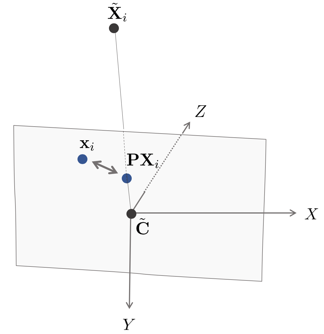
As in the method described above, if an over-determined linear system in the form of $\mathbf{Ap}=0$ is constructed using corresponding point pairs $(\mathbf{x}_{i}, \mathbf{X}_{i})$, an approximate solution vector $\hat{\mathbf{p}}$ that minimizes the size of $\| \mathbf{p} \|=1$이면서 $\| \mathbf{Ap} \|$ can be obtained. This section describes how to minimize the geometric error to obtain a more accurate camera matrix $\mathbf{P}$.The geometric error is the pixel distance between an already given $\mathbf{x}_{i}$ on the image plane and the projected $\mathbf{PX}_{i}$ of a point $\mathbf{X}_{i}$ on the world. In real data, $\mathbf{x}_{i} \neq \mathbf{PX}_{i}$ due to noise, so we need to find the optimal camera matrix $\mathbf{P}$ that minimizes the distance $d(\mathbf{x}_{i}, \mathbf{PX}_{i})$ between two points.
\begin{equation}
\begin{aligned}
\min_{\mathbf{P}} d(\mathbf{x}_{i}, \mathbf{PX}_{i})^{2}
\end{aligned}
\end{equation}
Since $d(\mathbf{x}_{i}, \mathbf{PX}_{i})^{2}$ is generally non-linear, the non-linear least squares methods Gauss-Newton( GN) or Levenberg-Marquardt (LM) method can be used to find the optimal camera matrix $\mathbf{P}$.
3.2.1. Algorithm 7.1
- Objective: For a given correspondence point pair $(\mathbf{x}_{i}, \mathbf{X}_{i}),\ i=1,\cdots,6,\cdots$, find the MLE (maximum likelihook estimation) value for $\mathbf{P}$. That is, find the camera matrix $\mathbf{P}$ that minimizes the $\sum_{i} d(\mathbf{x}_{i}, \mathbf{PX}_{i})^{2}$.
- Normalization: Image points $\mathbf{x}_{i}$ are normalized to $\mathbf{x}_{i} \rightarrow \bar{\mathbf{x}}_{i}$ through the normalizing matrix $\mathbf{T}$, and point $\mathbf{X}_{i}$ on the world is normalized to $\mathbf{X}_{i} \rightarrow \bar{\mathbf{X}}_{i}$ through the normalizing matrix $\mathbf{U}$. When direct linear transformation (DLT) is performed without normalization, the value of the last term is 1, which is very small due to the nature of the $\mathbb{P}^{2}$ and $\mathbb{P}^{3}$ spaces. The remaining terms are very large, so no appropriate solution is derived.
- DLT: The normalized pairs of correspondence points are composed of the above-described over-determined system $\bar{\mathbf{A}}\bar{\mathbf{p}}=0$. Next, after obtaining an approximate solution $\bar{\mathbf{p}}$ that is $\|\bar{\mathbf{p}} \|=1$ and minimizes $\|\bar{\mathbf{A}}\bar{\mathbf{p}}\|$ through DLT, set as the initial value $\bar{\mathbf{P}}_{0}$.
- Minimize geometric error: The following geometric errors are minimized by GN or LM methods to calculate the optimal normalized camera matrix $\bar{\mathbf{P}}$.
\begin{equation}
\begin{aligned}
\min_{\bar{\mathbf{P}}}\sum_{i} d(\bar{\mathbf{x}}_{i}, \bar{\mathbf{P}}\bar{\mathbf{X}}_{i})^{2} \quad \text{ start at } \bar{\mathbf{P}}_{0}
\end{aligned}
\end{equation}
- Denormalization: The normalized camera matrix is restored back to the original camera matrix.
\begin{equation}
\begin{aligned}
\mathbf{P} = \mathbf{T}^{-1}\bar{\mathbf{P}}\mathbf{U}
\end{aligned}
\end{equation}
The above algorithm is generally referred to as The Gold Standard algorithm for estimating $\mathbf{P}$. In practice, when using the above algorithm, a pair of corresponding points on the checkerboard is used instead of a random pair of matching points. The algorithm that estimates the camera matrix $\mathbf{P}$ through the checkerboard is called Zhang's Method..
3.3. Zhang's method

In practice, when using the Gold Standard algorithm, pairs of corresponding points on the checkerboard are used rather than random pairs of corresponding points. The algorithm for estimating the camera matrix $\mathbf{P}$ through the checkerboard is called Zhang's Method. Given the checkerboard plane $\pi_{0}$ in the world, set the origin in the world to the top left of the checkerboard and set the checkerboard plane to the plane $Z=0$.
\begin{equation}
\begin{aligned}
\pi_{0} = \{ \mathbf{X}=(X,Y,Z)^{\intercal} \ | \ Z=0 \}
\end{aligned}
\end{equation}
Accordingly, any point $\mathbf{X}_{i}$ on the checkerboard plane $\pi_{0}$ becomes a point with $Z=0$.
\begin{equation}
\begin{aligned}
\mathbf{X}_{i} = (\ast,\ \ast,\ 0)^{\intercal}
\end{aligned}
\end{equation}
Projecting a point on the checkerboard $\mathbf{X}=(X,\ Y,\ 0,\ 1)^{\intercal}$ gives:
\begin{equation}
\begin{aligned}
\mathbf{PX} & = \mathbf{P} \begin{pmatrix} X\\Y\\0\\1 \end{pmatrix} = \mathbf{K}[\mathbf{R} \ | \ \mathbf{t}] \begin{pmatrix} X\\Y\\0\\1 \end{pmatrix} \\
& = \mathbf{K}[\mathbf{r}_{1,col} \ \mathbf{r}_{2,col} \ \mathbf{t}]\mathbf{X}
\end{aligned}
\end{equation}
Since $z=0$, the third column vector of the matrix $\mathbf{R}$ is 0. Matrix $\mathbf{K}[\mathbf{r}_{1,col} \ \mathbf{r}_{2,col} \ \mathbf{t}] \in \mathbb{R}^{3\times 3}$ can be viewed as Homography $\mathbf{H}$ which transforms from the checkerboard plane $\pi_{0}$ to the image plane $\pi$. \begin{equation}
\begin{aligned}
\mathbf{H} = \mathbf{K}[\mathbf{r}_{1,col} \ \mathbf{r}_{2,col} \ \mathbf{t}]
\end{aligned}
\end{equation}
Since the checkerboard knows both the length and number of patterns, it automatically knows the points $\mathbf{x}_{i},i=1,\cdots$ on the checkerboard plane $\pi_{0}$. Next, by using the feature extraction algorithm, the point $\mathbf{x}^{\prime}_{i}, i=1,\cdots$ of $\pi_{0}$ seen on the image plane $\pi$ can be obtained. Accordingly, a correspondence point pair $\mathbf{x}_{i} \in \pi_{0} \leftrightarrow \mathbf{x}_{i}^{\prime} \in \pi$ can be obtained. Through this, Homography $\mathbf{H}$ going to $\pi_{0} \mapsto \pi$ is calculated as follows
\begin{equation}
\begin{aligned}
& \mathbf{H} = \begin{bmatrix} \mathbf{h}_{1,col} & \mathbf{h}_{2,col} & \mathbf{h}_{3,col} \end{bmatrix} = \mathbf{K} \begin{bmatrix} \mathbf{r}_{1,col} & \mathbf{r}_{2,col} & \mathbf{t} \end{bmatrix} \\
\end{aligned}
\end{equation}
Rearranging this:
\begin{equation}
\begin{aligned}
& \mathbf{K}^{-1}\begin{bmatrix} \mathbf{h}_{1,col} & \mathbf{h}_{2,col} & \mathbf{h}_{3,col} \end{bmatrix} = \begin{bmatrix} \mathbf{r}_{1,col} & \mathbf{r}_{2,col} & \mathbf{t} \end{bmatrix}
\end{aligned}
\end{equation}
Since the column vectors $\mathbf{r}_{1,col}$과 $\mathbf{r}_{2,col}$ of the orthogonal matrix $\mathbf{R}$ are orthogonal to each other, $\mathbf{r}_{1,col}^{\intercal}\mathbf{r}_{2,col}=0$ holds. If you use the corresponding constraints, $\mathbf{K}^{-1}\mathbf{h}_{1,col} = \mathbf{r}_{1,col}$ and $\mathbf{K}^{-1}\mathbf{h}_{2,col} = \mathbf{r}_{2,col}$, the following holds by the orthogonal condition
\begin{equation}
\label{eq:1386}
\begin{aligned}
\mathbf{h}_{1,col}^{\intercal}\mathbf{K}^{-\intercal}\mathbf{K}^{-1}\mathbf{h}_{2,col} = 0
\end{aligned}
\end{equation}
In addition, since it is $\mathbf{r}_{1,col}^{\intercal}\mathbf{r}_{1,col} = \mathbf{r}_{2,col}^{\intercal}\mathbf{r}_{2,col}$ except for the scale (up to scale) by the orthogonal matrix condition, the following formula holds
\begin{equation}
\label{eq:1395}
\begin{aligned}
& \mathbf{h}_{1,col}^{\intercal}\mathbf{K}^{-\intercal}\mathbf{K}^{-1}\mathbf{h}_{1,col} = \mathbf{h}_{2,col}^{\intercal}\mathbf{K}^{-\intercal}\mathbf{K}^{-1}\mathbf{h}_{2,col}
\end{aligned}
\end{equation}
From a single checkerboard picture, we can obtain the above two equations. A general camera calibration matrix $\mathbf{K}$ has 5 variables as shown below, so $\mathbf{K}^{-\intercal}\mathbf{K}^{-1}$ is also a matrix with 5 variables.
\begin{equation}
\begin{aligned}
\mathbf{K} = \begin{bmatrix} f_{x} & s & x_{0} \\ & f_{y} & y_{0} \\ &&1 \end{bmatrix}
\end{aligned}
\end{equation}
Therefore, given at least three homographies $\mathbf{H}_{j}, \ j=1,2,3$, $\mathbf{K}^{-\intercal}\mathbf{K}^{- 1}$ can be determined.
- Acquire at least three checkerboard images to find the matrix $\mathbf{K}$ with five parameters. Since you can get two equations per image, you need to acquire three or more. Homography $\mathbf{H}_{j},\ j=1,2,3$ can be obtained for each image, and formulas \eqref{eq:1386} and \eqref{eq:1395} are obtained.
- Set to $\mathbf{S} =\mathbf{K}^{-\intercal}\mathbf{K}^{-1}$. Perform Cholesky Decomposition or singular value decomposition (SVD) on matrix $\mathbf{S}$ to find $\mathbf{K}^{-1}$. Since the matrix $\mathbf{S}$ is symmetric and positive definite, it decomposes like $\mathbf{U}^{\intercal}\mathbf{DU}$, and a square root matrix of the diagonal matrix $\mathbf{D}$ exists.
\begin{equation}
\begin{aligned}
\text{SVD}(\mathbf{S}) = \mathbf{U}^{\intercal}\mathbf{D}\mathbf{U} = (\mathbf{U}\sqrt{\mathbf{D}})(\mathbf{U}\sqrt{\mathbf{D}})^{\intercal}
\end{aligned}
\end{equation}
Through this, $\mathbf{K}$ can be obtained.
- Calculate $\mathbf{r}_{1,col}, \mathbf{r}_{2,col}, \mathbf{t}$ through the $\mathbf{K}^{-1}\mathbf{H} = [\mathbf{r}_{1,col} \ \mathbf{r}_{2,col} \ \mathbf{t}]$ equation and then use the equation below.
\begin{equation}
\begin{aligned}
\mathbf{r}_{3,col} = \mathbf{r}_{1} \times \mathbf{r}_{2}
\end{aligned}
\end{equation}
In conclusion, through each Homography $\mathbf{H}_{j},\ j=1,2,3$, the rotation $\mathbf{R}$ and the translation $\mathbf{t}$ and the internal parameter matrix $\mathbf{K}$ can be obtained.
3.4. Radial distortion
Unlike the ideal pinhole camera model, real camera images contain radial distortion, so if you calibrate them right away, you cannot obtain accurate $\mathbf{R},\mathbf{t},\mathbf{K}$. If you perform calibration using an actual toolkit, you can obtain distortion parameters in addition to $\mathbf{R},\mathbf{t},\mathbf{K}$ obtained above. Corresponding parameters are parameters that correct the radial distortion of the image.
When the focal length $f$ is small, the Field of View (FOV) widens, and at this time, large radial distortion occurs near the edge of the image. Conversely, if the focal length $f$ is small, the FOV is small and distortion is relatively less.
Let $(\breve{u}, \breve{v})$ be a point on the image plane where distortion exists, and let $(u,v)$ be a point on the image plane where the distortion is corrected. The unit of the two points is $[pixel]$. Let $(\breve{x}, \breve{y})$ be a point on the normalized image plane where distortion exists, and let $(x,y)$ be the point where the distortion is corrected. The units of the two normalized points are $[mm]$. Normalized means that the origins of the image plane $u_{0} and v_{0} are all 0. Between the normalized points, the following equation holds
\begin{equation}
\begin{aligned}
& \breve{x} = x + x(k_{1}r^{2} + k_{2}r^{4}) \\
& \breve{y} = y + y(k_{1}r^{2} + k_{2}r^{4}) \quad \text{where, } r^{2} = x^{2} + y^{2}
\end{aligned}
\end{equation}
The value of $r^{2}$ means that the greater the distance from the origin, the greater the distortion. Re-expressing the normalized points as points on the image plane in pixels is:
\begin{equation}
\begin{aligned}
& \breve{u} = u_{0} + \alpha \breve{x} \\
& \breve{v} = v_{0} + \beta \breve{v} \\
\end{aligned}
\end{equation}
$u_{0} , v_{0}$ mean the origin of the image plane, and $\alpha$ and $\beta$ mean the coefficients that convert points in mm to pixel units. Therefore, the relationship between the distorted points and the actual points can be found by calculating the radial distortion parameters $k_{1}$ and $k_{2}$.
4. More Single View Geometry
4.1. Camera calibration and the image of the absolute conic
4.1.1. Result 8.15

When there is a camera $\mathbf{C}$ located at the origin, back-projecting a single point $\mathbf{x}$ creates a straight line $\mathbf{d}$ passing through the center of the camera. At this time, $\mathbf{ d} = \mathbf{K}^{-1}\mathbf{x}$.
\begin{equation}
\begin{aligned}
\mathbf{x} & = \mathbf{P} \begin{bmatrix} \lambda \mathbf{d} \\ 1 \end{bmatrix} \\
& = \mathbf{K} [ \mathbf{I} | 0 ] \begin{bmatrix} \lambda \mathbf{d} \\ 1 \end{bmatrix} = \mathbf{Kd} \\
\end{aligned}
\end{equation}
Therefore, the following formula holds.
\begin{equation}
\begin{aligned}
& \mathbf{x} = \mathbf{Kd} \\
& \mathbf{d} = \mathbf{K}^{-1}\mathbf{x}
\end{aligned}
\end{equation}

Back-projection of two points $\mathbf{x}_{1}$ and $\mathbf{x}_{2}$ on the image plane creates straight lines of $\mathbf{d}_{1}$ and $\mathbf{d}_{2}$, respectively. At this time, the angle formed by the two straight lines is as follows can be calculated together.
\begin{equation}
\begin{aligned}
\cos\theta & = \frac{\mathbf{d}_{1}^{\intercal}\mathbf{d}_{2}}{\sqrt{\mathbf{d}_{1}^{\intercal}\mathbf{d}_{1}}\sqrt{\mathbf{d}_{2}^{\intercal}\mathbf{d}_{2}}} = \frac{(\mathbf{K}^{-1}\mathbf{x}_{1})^{\intercal}(\mathbf{K}^{-1}\mathbf{x}_{2})}{\sqrt{(\mathbf{K}^{-1}\mathbf{x}_{1})^{\intercal}(\mathbf{K}^{-1}\mathbf{x}_{1})}\sqrt{(\mathbf{K}^{-1}\mathbf{x}_{2})^{\intercal}(\mathbf{K}^{-1}\mathbf{x}_{2})}} \\
& = \frac{\mathbf{x}_{1}^{\intercal}(\mathbf{K}^{-\intercal}\mathbf{K}^{-1})\mathbf{x}_{2}}{\sqrt{\mathbf{x}_{1}^{\intercal}\mathbf{K}^{-\intercal}\mathbf{K}^{-1}\mathbf{x}_{1}}\sqrt{\mathbf{x}_{2}^{\intercal}\mathbf{K}^{-\intercal}\mathbf{K}^{-1}\mathbf{x}_{2}}}
\end{aligned}
\end{equation}
$\mathbf{K}^{-\intercal}\mathbf{K}^{-1}$ means Image of Absolute Conic.
4.1.2. Result 8.16
When a point $\mathbf{x}$ is located on a straight line $\mathbf{l}$ in the image plane, the following formula holds between the point and the straight line.
\begin{equation}
\begin{aligned}
\mathbf{x}^{\intercal}\mathbf{l} =0
\end{aligned}
\end{equation}

When $\mathbf{l}$ is back-projected, plane $\pi$ is created, and when $\mathbf{x}$ is back-projected, $\mathbf{d}=\mathbf{K}^{-1}\mathbf{x}$ is created. Since $(\mathbf{K}^{-1}\mathbf{x})^{\intercal}\pi = 0$ holds between them, $\mathbf{x}^{\intercal}(\mathbf{K}^{-\intercal}\pi)=0$ also holds. In conclusion, according to the formula of $\mathbf{x}^{\intercal}\mathbf{l}=0$, the following formula is established.
\begin{equation}
\begin{aligned}
& \mathbf{K}^{-\intercal}\pi = \mathbf{l} \\
& \pi = \mathbf{K}^{\intercal}\mathbf{l}
\end{aligned}
\end{equation}
4.2. The image of the absolute conic
Assuming that there is an infinity point $\mathbf{X}_{\infty} = (\mathbf{d}^{\intercal}, 0)^{\intercal}$ located on $\pi_{\infty}$ when there is an infinity plane $\pi_{\infty}$, projecting it onto the camera $\mathbf{P}=\mathbf{KR}[\mathbf{I}|-\tilde{\mathbf{C}}]$ gives the following.
\begin{equation}
\begin{aligned}
\mathbf{x} = \mathbf{PX}_{\infty} = \mathbf{KR}[\mathbf{I} | -\tilde{\mathbf{C}}] \begin{bmatrix} \mathbf{d} \\0 \end{bmatrix} = \mathbf{KRd}
\end{aligned}
\end{equation}
In other words, assuming that $\mathbf{x} = \mathbf{Hd}$ homography exists for the point $\mathbf{d}$ on the infinity plane $\pi_{\infty}$, the homography $\mathbf{H}$ is equal to $\mathbf{H}$는 $\mathbf{H}=\mathbf{KR}$. Absolute Conic $\Omega_{\infty}$ located at infinity is $\mathbf{I}_{3}\in \pi_{\infty}$. Homography conversion of $\Omega_{\infty}$ gives the following formula
\begin{equation}
\begin{aligned}
\mathbf{H}(\Omega_{\infty}) & = \mathbf{H}^{-\intercal}\mathbf{I}_{3}\mathbf{H}^{-1} \\
& = (\mathbf{KR})^{-\intercal}\mathbf{I}_{3}(\mathbf{KR})^{-1} \\
& = \mathbf{K}^{-\intercal}\mathbf{R}^{-\intercal}\mathbf{R}^{-1}\mathbf{K}^{-1} \\
& = \mathbf{K}^{-\intercal}\mathbf{K}^{-1}
\end{aligned}
\end{equation}
4.2.1. Result 8.17
Accordingly, Image of Absolute Conic is $\mathbf{w} = \mathbf{K}^{-\intercal}\mathbf{K}^{-1}$. When back-projecting two points $\mathbf{x}_{1}$ and $\mathbf{x}_{2}$ on the image, the angle formed by the two straight lines is as follows
\begin{equation}
\begin{aligned}
\cos\theta = \frac{\mathbf{x}_{1}^{\intercal}\mathbf{w}\mathbf{x}_{2}}{\sqrt{\mathbf{x}_{1}^{\intercal}\mathbf{w}\mathbf{x}_{1}}\sqrt{\mathbf{x}_{2}^{\intercal}\mathbf{w}\mathbf{x}_{2}}}
\end{aligned}
\end{equation}
The homography conversion of this is as follows.
\begin{equation}
\begin{aligned}
\cos\theta = \frac{(\mathbf{Hx}_{1})^{\intercal}\mathbf{H}^{-\intercal}\mathbf{w}\mathbf{H}^{-1}(\mathbf{Hx}_{2})}{\sqrt{\ast}\sqrt{\ast}}
\end{aligned}
\end{equation}
Therefore, even after homography conversion, the two angles are still preserved. If two straight lines $\mathbf{K}^{-1}\mathbf{x}_{1}$ and $\mathbf{K}^{-1}\mathbf{x}_{2}$ are orthogonal The following formula holds.
\begin{equation}
\begin{aligned}
\mathbf{x}_{1}^{\intercal}\mathbf{w}\mathbf{x}_{2} = 0
\end{aligned}
\end{equation}
4.3. Orthogonality and $\mathbf{w}$

Back-projecting two points $\mathbf{x}_{1}$ and $\mathbf{x}_{2}$ on the image plane gives two straight lines $\mathbf{K}^{-1}\mathbf{x }_{1}, \mathbf{K}^{-1}\mathbf{x}_2$ is created. If the two straight lines are orthogonal, the formula $\mathbf{x}_{1}^{\intercal}\mathbf{w}\mathbf{x}_{2}=0$ holds. And if $\mathbf{x}_{1}$ is included in the straight line $\mathbf{l}$, $\mathbf{x}_{1}^{\intercal}\mathbf{l}=0$ is established.
4.3.1. Result 8.19
Combining the above two formulas gives
\begin{equation}
\begin{aligned}
& \mathbf{x}_{1}^{\intercal}\mathbf{w}\mathbf{x}_{2}=0 \\
& \mathbf{x}_{1}^{\intercal}\mathbf{l} = 0 \\
& \therefore \mathbf{l} = \mathbf{wx}_{2}
\end{aligned}
\end{equation}
4.4. Vanishing points and vanishing lines

When a point $\mathbf{A}$ in 3D space and the direction $\mathbf{D}=(\mathbf{d}^{\intercal},0)^{\intercal}$ exist, the line exists The point $\mathbf{X}(\lambda)$ is defined as
\begin{equation}
\begin{aligned}
\mathbf{X}(\lambda) = \mathbf{A} + \lambda \mathbf{D} = \begin{bmatrix} \tilde{\mathbf{A}} + \lambda \mathbf{d} \\ 1 \end{bmatrix}
\end{aligned}
\end{equation}
Projection of point $\mathbf{X}(\lambda)$ onto image plane $\mathbf{x}(\lambda) = \mathbf{PX}(\lambda), \ \ \text{where } \ \mathbf {P} = \mathbf{K}[\mathbf{I}|0]$ is defined as:\begin{equation}
\begin{aligned}
\mathbf{x}(\lambda) = \mathbf{PX}(\lambda) = \mathbf{PA} + \lambda \mathbf{PD} = \mathbf{a} + \lambda \mathbf{Kd}
\end{aligned}
\end{equation}
$\mathbf{a}$ means Image of $\mathbf{A}$.
4.4.1. Result 8.20
In conclusion, the vanishing point $\mathbf{v}$ is defined as
\begin{equation}
\begin{aligned}
& \mathbf{v} = \lim_{\lambda \rightarrow \infty}\mathbf{x}(\lambda) = \lim_{\lambda \rightarrow \infty}(\mathbf{a} + \lambda \mathbf{Kd}) = \mathbf{Kd} \\
& \mathbf{v} = \mathbf{Kd}
\end{aligned}
\end{equation}
4.4.2. Camera rotation from vanishing points
You can use the vanishing point to calculate the rotation of the camera. When there is a vanishing point $\mathbf{v}_{1}$ extracted from image 1 and a vanishing point $\mathbf{v}_{2}$ extracted from image 2, the direction of $\mathbf{v}_{1}$ becomes $\mathbf{d}_{1} = \mathbf{K}^{-1}\mathbf{v}_{1}$ and the direction of $\mathbf{v}_{2}$ becomes $\mathbf{d}_{2} = \mathbf{K}^{-1}\mathbf{v}_{2}$.
Assuming that the values of $\mathbf{K}, \mathbf{v}_{1}$ and $\mathbf{v}_{2}$ are known, the value of $\mathbf{d}_{1}, \mathbf{d}_{2}$ can be calculated, and the two direction vectors are have the same relationship as
\begin{equation}
\begin{aligned}
\mathbf{d}_{2} = \mathbf{Rd}_{1}
\end{aligned}
\end{equation}
Since the degree of freedom of the rotation matrix $\mathbf{R}$ is 3, the rotation matrix can be restored by using two or more vanishing point pairs.
4.5. Vanishing Lines

A straight line connecting two or more vanishing points $\mathbf{v}_{i}, i=1,2,\cdots$ is called a vanishing line $\mathbf{l}$. For example, consider a case where there is a checkerboard on the image and two vanishing points $\mathbf{v}_{1} , \mathbf{v}_{2}$ are obtained because of this. In this case, the straight line $\mathbf{l}$ connecting the two vanishing points $\mathbf{v}_{1},\mathbf{v}_{2}$ is called the vanishing line of the checkboard plane $\pi$.
\begin{equation}
\begin{aligned}
\mathbf{l} = \text{image of } \pi \cap \pi_{\infty}
\end{aligned}
\end{equation}
In conclusion, the vanishing line $\mathbf{l}$ means the intersection of the image plane with the plane $\pi^{\prime}$ that includes the camera center and is parallel to the checkerboard plane $\pi$. $\pi^{\prime}$ can be calculated by back-projecting the vanishing line $\mathbf{l}$. At this time, the following formula is established according to the relationship between the plane and the straight line.
\begin{equation}
\begin{aligned}
\pi^{\prime} = \mathbf{K}^{\intercal}\mathbf{l}
\end{aligned}
\end{equation}
4.6. Orthogonality relationships amongst vanishing points and lines

The condition that the straight lines back-projected from the two vanishing points $\mathbf{v}_{1}$ and $\mathbf{v}_{2}$ on the image plane are orthogonal to each other is as follows.
\begin{equation}
\begin{aligned}
\mathbf{v}_{1}^{\intercal}\mathbf{w}\mathbf{v}_{2} = 0
\end{aligned}
\end{equation}
$\mathbf{w} = \mathbf{K}^{-\intercal}\mathbf{K}^{-1}$ is the Image of Absolute Conic. The condition that the straight line back-projected by the vanishing point $\mathbf{v}$ on the image plane and the plane back-projected by the vanishing line $\mathbf{l}$ are orthogonal are as follows.
\begin{equation}
\begin{aligned}
\mathbf{l} = \mathbf{w}\mathbf{v}
\end{aligned}
\end{equation}
When two planes back-projected by two straight lines $\mathbf{l}_{1}$ and $\mathbf{l}_{2}$ on the image plane are orthogonal to each other, the following is satisfied.
\begin{equation}
\begin{aligned}
\mathbf{l}_{1}^{\intercal}\mathbf{w}^{\ast}\mathbf{l}_{2} =0
\end{aligned}
\end{equation}
$\mathbf{w}^{\ast}$ is the Image of Dual Absolute Conic.
4.7. Affine 3D measurements and reconstruction

The vanishing point of objects perpendicular to the plane $\pi$ in 3D space is called the vertical vanishing point $\mathbf{v_{\perp}}$.
4.7.1. Result 8.24
Using the vanishing line $\mathbf{l}$ of the plane $\pi$ and the vertical vanishing point, the size of the object can be calculated up to the parameters (up to scale) except for the scale. To be precise, if we know the vanishing line $\mathbf{l}$ and the vertical vanishing point $\mathbf{v}_{\perp}$, we can find the relative lengths of the lines perpendicular to the plane $\pi$.
For example, suppose there are two points $\mathbf{B}_{1}$ and $\mathbf{B}_{2}$ located on plane $\pi$ in 3D space. Also, suppose there are straight lines $\mathbf{L}_{1}$ and $\mathbf{L}_{2}$ perpendicular to the plane $\pi$ passing through them. And if there are end points $\mathbf{T}_{1}, \mathbf{T}_{2}$ of two straight lines $\mathbf{L}_{1}, \mathbf{L}_{2}$ , using the vanishing line $\mathbf{l}$ and the vertical vanishing point $\mathbf{v}_{\perp}$, Relative lengths can be measured.
First, all elements are projected onto the image plane. At this time, the point where the straight line connecting $\mathbf{b}_{1}, \mathbf{b}_{2}$ and the vanishing line $\mathbf{l}$ meet is defined as $\mathbf{u}$. And if you draw a straight line parallel to $\bar{\mathbf{b}_{1}\mathbf{b}_{2}}$ from $\mathbf{t}_{1}$, the straight line touches $\mathbf{u}$. At this time, the intersection of $\bar{\mathbf{t}_{1}\mathbf{u}}$ and $\mathbf{v}_{\perp}\mathbf{b}_{2}$ is called $\tilde{\mathbf{t}}_{1}$.
Next, the $\bar{\mathbf{v}_{\perp}\mathbf{b}_{2}}$ straight line is converted to the vertical vanishing point of $\mathbb{P}^{1}$ space $\mathbf{v} _{\perp}$ becomes the point $(1,0)$ of infinity, and $\mathbf{b}_{1}$ is projected as a straight line with the origin $(0,1)$. The Homography $\mathbf{H}_{2\times2}$ used at this time is as follows.
\begin{equation}
\begin{aligned}
\mathbf{H}_{2\times2} = \begin{bmatrix} 1 & 0 \\ 1 & -\mathbf{v}_{\perp} \end{bmatrix}
\end{aligned}
\end{equation}
$\mathbf{H}_{2\times2}$ guarantees the Cross-Ratio. Next, the ratio of $d_{1} : d_{2} = \mathbf{b}_{1}\tilde{\mathbf{t}}_{1}:\mathbf{b}_{1}\mathbf{t}_{2}$ is obtained using the ratio of the lengths.
\begin{equation}
\begin{aligned}
\frac{d_{1}}{d_{2}} = \frac{\tilde{\mathbf{t}}_{1}(\mathbf{v}_{\perp}-\mathbf{t}_{2})}{\mathbf{t}_{2}(\mathbf{v}_{\perp}-\tilde{\mathbf{t}}_{1})}
\end{aligned}
\end{equation}
If the vertical vanishing point $\mathbf{v}_{\perp}$ and the principal axis of the camera are perpendicular, the vertical vanishing point does not meet on the image and the ratio can be calculated simply as follows.
\begin{equation}
\begin{aligned}
\frac{d_{1}}{d_{2}} = \frac{\tilde{\mathbf{t}}_{1}-\mathbf{b}_{2}}{\mathbf{t}_{2}-\mathbf{b}_{2}}
\end{aligned}
\end{equation}
4.8. Determining camera calibration $\mathbf{K}$ from a single view
Two constraints are needed to determine the internal parameter $\mathbf{K}$ in the monocular image. There are scene constraints and internal parameter constraints.
As an image constraint condition, if there are two mutually perpendicular vanishing points $\mathbf{v}_{1}, \mathbf{v}_{2}$ existing on the image plane, $\mathbf{v}_{1}^{\intercal}\mathbf{w}\mathbf{v}_{2}=0$ is satisfied, and if the vanishing line $\mathbf{l}$ and the vanishing point $\mathbf{v}$ are orthogonal, their back-projection becomes $\mathbf{l} = \mathbf{wx}$.
\begin{equation}
\begin{aligned}
& \mathbf{v}_{1}^{\intercal}\mathbf{w}\mathbf{v}_{2}=0 \\
& \mathbf{l} \times (\mathbf{wv}) = 0
\end{aligned}
\end{equation}
4.8.1. Result 8.26
Internal parameter constraints include $w_{12} = w_{21} = 0$ when $\mathbf{K}$ is Zero-Skew, and $w_{12}=w_{21}=0, w_{11}=w_{22}$ when $\mathbf{K}$ is Square Pixels.
\begin{equation}
\begin{aligned}
& w_{12} = w_{21} \quad \text{for zero skew} \\
& w_{12}=w_{21}=0, w_{11}=w_{22} \quad \text{for square pixel}
\end{aligned}
\end{equation}
After securing enough constraints to find the $\mathbf{w} = \begin{bmatrix} w_{1} & w_{2} & w_{4} \\ w_{2} & w_{3} &w_{5} \\ w_{4} & w_{5} & w_{6} \end{bmatrix}$ parameters as above, $\mathbf{w}$ is sorted into a 6-dimensional vector to create a linear system of the form $\mathbf{Ax}=0$. Next, we use Singular Value Decomposition (SVD) to calculate $\mathbf{w}=\mathbf{K}^{-\intercal}\mathbf{K}^{-1}$ values, and then Cholesky Decomposition to decompose the $\mathbf{K}^{-\intercal}\mathbf{K}^{-1}$. With this, the internal parameter $\mathbf{K}$ can be calculated.
4.9. Calibration from three orthogonal vanishing points

When the internal parameter $\mathbf{K}$ is Zero-Skew and Square Pixel, $\mathbf{K}$ can be calculated using three mutually orthogonal vertical vanishing points $\mathbf{v}_{i}, \ i=1,2,3$. First of all, since $\mathbf{K}$ is Zero-Skew and Square Pixel, the following holds.
\begin{equation}
\begin{aligned}
\mathbf{w} = \begin{bmatrix} w_{1} & 0 & w_{2} \\ 0 & w_{1} & w_{3} \\ w_{2} & w_{3} & w_{4} \end{bmatrix}
\end{aligned}
\end{equation}
As such, since it has a total of four degrees of freedom, $\mathbf{K}$ can be determined using three vertical vanishing points. First, $\mathbf{v}_{i}^{\intercal}\mathbf{w}\mathbf{v}_{j}, \ \forall i\neq j$ is calculated using the orthogonal characteristics of each vertical vanishing point. At this time, $\mathbf{w}$ is vectorized, converted into a linear system of the form $\mathbf{Ax}=0$, and $\mathbf{w}$ is obtained by calculating Nul $(\mathbf{A})$. Next, the $\mathbf{w}=\mathbf{K}^{-\intercal}\mathbf{K}^{-1}$ is decomposed using Cholesky Decomposition. In this way, the internal parameter $\mathbf{K}$ can be calculated.
4.10. Computation of focal length and principal point using vanishing point and vanishing line

If there is a vanishing line $\mathbf{l}$ that can be obtained from a plane $\pi$ in 3D space and there is a vertical vanishing point $\mathbf{v}_{\perp}$ perpendicular to $\pi$, the focal length f and the principal point can be obtained using this.
The method of calculating the focal length f is as follows. Let the vertical vanishing point be $\mathbf{v}_{\perp}$ and the line of intersection of image plane $\pi_{\mathbf{C}}$ and plane $\pi$ be $\mathbf{l}$, let $\mathbf{v}_{\perp}\tilde{\mathbf{C}}$ and $\mathbf{x}\tilde{\mathbf{C}}$ are orthogonal to each other. And if there is a point P that is perpendicular to the image plane from the center of the camera, the length of $\tilde{\mathbf{C}}\mathbf{p}$ is the focal length f. After drawing a circle whose diameter is $\mathbf{v}_{\perp}x$, let $\mathbf{a}$ and $\mathbf{b}$ be the point of intersection of the circle and the line drawn horizontally at the point $\mathbf{p}$. It becomes the center $\tilde{\mathbf{C}}$, which means that $\mathbf{ap} = \mathbf{bp}$ is the focal length f.
The method for obtaining the principal point P is as follows. If the vertical vanishing point is $\mathbf{v}_{1}$ and the line of intersection of the image plane and the $\pi$ plane is $\mathbf{l}_{1}$, then if $\mathbf{v}_{1}$ lowers the normal to $\mathbf{l}_{1}$, the principal point $\mathbf{p}$ is located Due to this feature, if there are three different vertical vanishing points, the orthocenter of the triangle becomes the principal point $\mathbf{p}$.
4.11. The calibrating conic

Image of absolute conic (IAC) is a useful tool that can find the angle between straight lines that back-projected points on the image plane and perform metric rectification. However, due to the nature of Circular Point, it has a disadvantage that it is impossible to visualize because it does not have a root of a real number. Calibration Conic was devised to supplement this. Calibration Conic means Image Conic projected with Cone of $X^{2}+Y^{2}=Z^{2}$ and has the advantage of being able to visualize.
Given the camera projection $\mathbf{P} = \mathbf{K}[\mathbf{I}|0]$ the points on the Calibration Conic are projected as:
\begin{equation}
\begin{aligned}
\mathbf{C} = \mathbf{K}^{-\intercal}\begin{bmatrix} 1 & & \\ & 1 & \\ & & -1 \end{bmatrix}\mathbf{K}^{-1}
\end{aligned}
\end{equation}
At this time, $\mathbf{D}= \begin{bmatrix} 1 & & \\ & 1 & \\ & & -1 \end{bmatrix}$ can be expressed as $\mathbf{C} = \mathbf{K}^{-\intercal}\mathbf{D}\mathbf{K}^{-1}$. If it is $\mathbf{K} = \begin{bmatrix} f & & \\ & f & \\ & & 1 \end{bmatrix}$, Calibration Conic can be expressed as follows.
\begin{equation}
\begin{aligned}
\mathbf{C} = \begin{bmatrix} 1 & & \\ & 1 & \\ & & -f^{2} \end{bmatrix}
\end{aligned}
\end{equation}
Calibration Conic means a circle on an image whose origin is the principal point and whose radius is the focal length f. Decomposition of $\mathbf{C}$ can be redefined as follows.
\begin{equation}
\begin{aligned}
& \mathbf{C} = \mathbf{K}^{-\intercal}\mathbf{DK}^{-1} = \mathbf{K}^{-\intercal}\mathbf{K}^{-1}\mathbf{KDK}^{-1} \\
& \mathbf{C} = \mathbf{w}\mathbf{S} \quad \text{where, } \mathbf{S} = \mathbf{KDK}^{-1}
\end{aligned}
\end{equation}

For a random point $\mathbf{x}=\mathbf{K}\tilde{\mathbf{X}}$ on the image, $\mathbf{Sx}$ means a point reflected by Calibration Conic.
\begin{equation}
\begin{aligned}
\mathbf{Sx} & = \mathbf{KDK}^{-1}\mathbf{K}\tilde{\mathbf{X}} \\
& = \mathbf{KD}\begin{bmatrix} X \\ Y \\ Z \end{bmatrix} = \mathbf{K}\begin{bmatrix} X \\ Y \\ -Z \end{bmatrix}
\end{aligned}
\end{equation}
For two points $\mathbf{x}, \mathbf{x}^{\prime}$ on the image plane, if the back-projected straight lines of the two points are orthogonal to each other, $\mathbf{x}^{\prime\intercal}\mathbf{wx}=0$ is established. Rewriting this expression gives:
\begin{equation}
\begin{aligned}
& \mathbf{x}^{\prime\intercal}\mathbf{wx} = \mathbf{x}^{\prime\intercal}\mathbf{CS}^{-1}\mathbf{x} = \mathbf{x}^{\prime\intercal}\mathbf{CSx} = \mathbf{x}^{\prime\intercal}\mathbf{C}\dot{\mathbf{x}} \\
& \because \mathbf{S}^{-1} = \mathbf{S}
\end{aligned}
\end{equation}
At this time, $\dot{\mathbf{x}} = \mathbf{Sx}$ means the point where $\mathbf{x}$ is reflected by Calibration Conic.
4.11.1. Result 8.30
In conclusion, the straight line $\mathbf{C}\dot{\mathbf{x}}$ becomes a straight line connecting the tangents of the reflected point $\dot{\mathbf{x}}$ and Calibration Conic, and the point $\mathbf{x}^{\prime}$ exists on the straight line $\mathbf{C}\dot{\mathbf{x}}$.
5. References
'English' 카테고리의 다른 글
| [SLAM][En] Direct Sparse Odometry (DSO) Paper Review Part 2 (0) | 2023.01.17 |
|---|---|
| [SLAM][En] Direct Sparse Odometry (DSO) Paper Review Part 1 (0) | 2023.01.17 |
| [En] Notes on Lie Theory (SO(3), SE(3)) (0) | 2023.01.17 |
| [En] Notes on Plücker Coordinate (0) | 2023.01.17 |
| [SLAM][En] Errors and Jacobian Derivations for SLAM Part 2 (0) | 2023.01.17 |


