 A L I D A
1. Introduction
The Plücker Coordinate representation was first introduced by the 19th century mathematician Julius Plücker. This expression is one of the ways to express a line, and is used to express a line in the 4-dimensional $\mathbb{P}^{3}$ space using a point in the 6-dimensional $\mathbb{P}^{5}$ space. do. This expression method is characterized by a one-to-one correspondence between a point on the $\mathbb{P}^{5}$ quadric and a line on the $\mathbb{P}^{3}$ space due to its own constraints. For more information on projective space, see this post.
In MVG books, a point in 3D space is usually expressed as $\mathbf{X} = [X,Y,Z,W] \in \mathbb{P}^{3}$, but in Plücker Coordinates (\ref{ Like eq:2}), the $[W,X,Y,Z]$ is sometimes used for the convenience of $l_{ij}$ indexing. When expressed in the order of $[X,Y,Z,W]$, it is equivalent to (\ref{eq:3}). Therefore, when using them in practice, care must be taken in order.
In the field of computer graphics, the Plücker Coordinate expression method is often used, and in robotics and kinematics, the line expression method is often used when expressing screws and wrenches. In addition, in the SLAM field, when using lines, you can also see research on tracking line features or performing optimization using the Plücker Coordinate expression method [4][5].
NOMENCLATURE
- A Plücke line in three-dimensional space is denoted by $\mathcal{L} \in \mathbb{P}^{5}$.
- line on the image plane is denoted by $l \in \mathbb{P}^{2}$. Note in this post that $l$ is not a scalar.
- The Plücker matrix is denoted $\mathbf{L} \in \mathbb{R}^{6\times 6}$. Note that this is a 6x6 matrix and not a Plücke line.
- The Plücker matrix of line on the image plane is denoted $\mathbf{l} \in \mathbb{R}^{3\times 3}$. Note that this is not line, but a 3x3 matrix.
- $(*)^{\wedge}$ means the skew-symmetric matrix of the vector $*$ e.g., $\mathbf{x} = \begin{bmatrix} x,y,z \end{bmatrix}^{\intercal}$일 때 $\mathbf{x}^{\wedge} = \begin{bmatrix} 0 & -z & y \\ z & 0 & -x \\ -y & x & 0 \end{bmatrix}$. In other documents, it is also written as $[*]_{\times}$.
2. How to represent a line in 3D space

There are several ways to express a line in a 3D space. For example, the line $\mathcal{L}$ can be expressed by using two points $\mathbf{p}_{1}$ and $\mathbf{p}_{2}$.
\begin{equation}
\begin{aligned}
\mathcal{L} (\mathbf{p}_{1}, \mathbf{p}_{2})
\end{aligned}
\end{equation}
Alternatively, a line can be expressed with $\mathbf{p}_{1}$ and a direction vector $\mathbf{d}$, a point on the line.
\begin{equation}
\begin{aligned}
& \mathcal{L} (\mathbf{p}_{1}, \mathbf{d}) \\
& \text{where, } \mathbf{d} = \mathbf{p}_{2} - \mathbf{p}_{1} \\
\end{aligned}
\end{equation}

Alternatively, since the intersection of two non-parallel planes $\pi_{1}$ and $\pi_{2}$ forms a line, the line $\mathcal{L}$ can be expressed through the two planes.
\begin{equation}
\begin{aligned}
\mathcal{L} (\pi_{1}, \pi_{2})
\end{aligned}
\end{equation}

Alternatively, a line can be expressed using the direction vector $\mathbf{d}$ of the line and the direction vector $\mathbf{m}$ of the plane $\pi_{0}$ including the origin and containing the line.
\begin{equation}
\begin{aligned}
& \mathcal{L} (\mathbf{d}, \mathbf{m}) \in \mathbb{P}^{5} \\
& \text{where, } \mathbf{d} = \mathbf{p}_{2} - \mathbf{p}_{1} \\
& \mathbf{m} = \mathbf{p}_{1} \times \mathbf{p}_{2}
\end{aligned}
\end{equation}
At this time, $\mathbf{m}$ can be thought of as a moment vector that occurs when a point $\mathbf{p}_{1}$ with unit mass moves in $\mathbf{p}_{2}$. The magnitude of the moment vector is twice the area of the triangle connecting $\mathbf{p}_{1}, \mathbf{p}_{2}$ and the origin. Since the direction vector $\mathbf{d}$ and the moment vector $\mathbf{m}$ are orthogonal to each other, the following formula holds.
\begin{equation}
\begin{aligned}
& \mathbf{m}^{\intercal} \cdot \mathbf{d} = 0
\end{aligned} \label{eq:4}
\end{equation}
The line $\mathcal{L}$ cannot be uniquely expressed using either $\mathbf{d}$ or $\mathbf{m}$, but the $(\mathbf{d}, \mathbf{m})$ pair can express a unique line independent of scalar values (up to scale).
\begin{equation}
\begin{aligned}
(\mathbf{d}:\mathbf{m}) = (d_{x}:d_{y}:d_{z}:m_{x}:m_{y}:m_{z})
\end{aligned}
\end{equation}
Among these various line expression methods, the method of expressing a line using $(\mathbf{d},\mathbf{m})$ is called the Plücker Coordinate expression method. Since this expression is a homogeneous expression, it satisfies $(\mathbf{d}:\mathbf{m}) = (\lambda\mathbf{d}:\lambda\mathbf{m})$ for a non-zero scalar $\lambda$.
3. Plücker coordinate representation
The method of expressing a line in Plücker Coordinate is as follows. When two points $\mathbf{p}_{1}$ and $\mathbf{p}_{2}$ exist in $\mathbb{P}^{3}$ space, it can be expressed as follows.
\begin{equation}
\begin{aligned}
& \mathbf{p}_{1} = [W_{1}, X_{1}, Y_{1}, Z_{1}] \\
& \mathbf{p}_{2} = [W_{2}, X_{2}, Y_{2}, Z_{2}]
\end{aligned}
\end{equation}
For convenience of explanation, it is written in the order of $[X, Y, Z, W] \rightarrow [W, X, Y, Z]$. When there is a direction vector $\mathbf{d} = \mathbf{p}_{2} - \mathbf{p}_{1}$ for a line and a direction vector $\mathbf{m}=\mathbf{p}_{2}\times \mathbf{p}_{1}$ of the plane containing the origin and the line, the line $\mathcal{L}$ can be expressed as follows.
\begin{equation}
\begin{aligned}
\mathcal{L} = (\mathbf{d}:\mathbf{m}) = (d_{x}:d_{y}:d_{z}:m_{x}:m_{y}:m_{z})
\end{aligned}
\end{equation}
At this time, $\mathbf{m}$ is the moment vector between the origin and the line, and if the moment vector is 0, it means that the line includes the origin. In order to derive the value of the above expression, if a matrix $\mathbf{M} \in \mathbb{R}^{2\times 4}$ with two points as rows is set as follows and the determinant operation $l_{ij}$ for a 2x2 submatrix is defined, it is as follows.
\begin{equation}
\begin{aligned}
& \mathbf{M} = \begin{bmatrix} W_{1} & X_{1} & Y_{1} & Z_{1} \\ W_{2}&X_{2}&Y_{2}&Z_{2} \end{bmatrix} \\
& l_{ij} = \begin{vmatrix} X_{i} & Y_{i} \\ X_{j} & Y_{j} \end{vmatrix} = X_{i}Y_{j} - X_{j}Y_{i}
\end{aligned}
\end{equation}
It has the characteristics of $l_{ii}=0, l_{ij} = -l_{ji}$. In conclusion, the line $\mathcal{L}$ can be defined as follows.\begin{equation}
\begin{aligned}
\mathcal{L} = (\mathbf{d}:\mathbf{m}) & = (d_{x}:d_{y}:d_{z}:m_{x}:m_{y}:m_{z}) \\ &= (l_{01}:l_{02}:l_{03}:l_{23}:l_{31}:l_{12})
\end{aligned} \label{eq:2}
\end{equation}
The line expression method can only express a line except for scale (up to scale), and at least one element must be non-zero. In general, Plücker Coordinate expresses a point in $\mathbb{P}^{5}$ space, which is homogeneous, using a colon (:). The reason why the colon (:) is used is that the ratio between the elements is more important than the value itself of the six elements in terms of up to scale characteristics.
At this time, each component of $l_{ij}$ is described in detail as follows.
\begin{equation}
\begin{aligned}
& l_{01} = W_{1}X_{2}-W_{2}X_{1} & l_{23} = Y_{1}Z_{2}-Z_{1}Y_{2} \\
& l_{02} = W_{1}Y_{2}-W_{2}Y_{1} &l_{31} = Z_{1}X_{2}-X_{1}Z_{2} \\
& l_{03} = W_{1}Z_{2}-W_{2}Z_{1} & l_{12} = X_{1}Y_{2}-Y_{1}X_{2}
\end{aligned}
\end{equation}
\begin{equation}
\begin{aligned}
\mathbf{d} = \begin{bmatrix} W_{1}X_{2}-W_{2}X_{1} \\
W_{1}Y_{2}-W_{2}Y_{1} \\
W_{1}Z_{2}-W_{2}Z_{1} \end{bmatrix} \quad \quad
\mathbf{m} = \begin{bmatrix} Y_{1}Z_{2}-Z_{1}Y_{2} \\
Z_{1}X_{2}-X_{1}Z_{2} \\
X_{1}Y_{2}-Y_{1}X_{2} \end{bmatrix}
\end{aligned}
\end{equation}
At this time, from the above expression, $\mathbf{m} = \mathbf{p}_{1} \times \mathbf{p}_{2}$. If $W_{1}=W_{2}=1$, $l_{01}, l_{02}$, and $l_{03}$ can be concisely expressed as follows.
\begin{equation}
\begin{aligned}
l_{01} = X_{2}-X_{1} \quad l_{02} = Y_{2}-Y_{1} \quad l_{03} = Z_{2}-Z_{1}
\end{aligned}
\end{equation}
This is equivalent to the definition of $\mathbf{d} = \mathbf{p}_{2} - \mathbf{p}_{1}$.
3.1. Graßmann–Plücker relations
In the Plücker Coordinates representation, there is a one-to-one correspondence between a point on the $\mathbb{P}^{5}$ quadric and a line on the $\mathbb{P}^{3}$ space due to a constraint called the Graßmann-Plücker relations. There are features that make up At this time, the $\mathbb{P}^{5}$ curved surface corresponding to the line in the $\mathbb{P}^{3}$ space is specially called a Klein quadric and satisfies the following constraints.
\begin{equation}
\begin{aligned}
l_{01}l_{23} + l_{02}l_{31} + l_{03}l_{12} = 0
\end{aligned}
\end{equation}
Or, since $l_{31} = -l_{13}$, we can write:
\begin{equation}
\begin{aligned}
l_{01}l_{23} - l_{02}l_{13} + l_{03}l_{12} = 0
\end{aligned}
\end{equation}
The above expression is derived from (\ref{eq:4}) $\mathbf{m}^{\intercal}\mathbf{d} = 0$ and can also be obtained through $\det \mathbf{L} = 0$ .
3.2. Distance to origin

The distance the line is from the origin $\left\| \mathbf{p}_{\perp} \right\|$ can be obtained as follows. If an arbitrary point $\mathbf{q}$ on the line $\mathcal{L}$ is given and $\mathbf{p}_{\perp}$ is the point where the perpendicular of the line descends from the origin, $\mathbf{p}_{\perp}$ can be expressed through $\mathbf{q}$.
\begin{equation}
\begin{aligned}
\mathbf{q} = \mathbf{p}_{\perp} + k\mathbf{d} \quad (\text{any } \mathbf{q} \text{ on } \mathcal{L})
\end{aligned}
\end{equation}
Accordingly, the moment vector $\mathbf{m}$ can be expanded as follows.
\begin{equation}
\begin{aligned}
\mathbf{m} & = \mathbf{d} \times \mathbf{q} \\
& = \mathbf{d} \times (\mathbf{p}_{\perp} + k\mathbf{d}) \\
& = \mathbf{d} \times \mathbf{p}_{\perp}
\end{aligned}
\end{equation}
According to the definition of the magnitude cross product of moment vectors, it can be expressed as follows.
\begin{equation}
\begin{aligned}
\left\| \mathbf{m} \right\| = \left\| \mathbf{d} \right\|\left\| \mathbf{p}_{\perp} \right\|\sin\frac{\pi}{2} = \left\| \mathbf{d} \right\|\left\| \mathbf{p}_{\perp} \right\|
\end{aligned}
\end{equation}
Therefore, the distance from the origin to the line $\mathcal{L}$ is:
\begin{equation}
\begin{aligned}
\left\| \mathbf{p}_{\perp} \right\| = \frac{\left\| \mathbf{m} \right\|}{\left\| \mathbf{d} \right\|}
\end{aligned}
\end{equation}
3.3. Up to scale uniqueness

If there is any other point $\mathbf{p}^{\prime}_{1}, \mathbf{p}^{\prime}_{2}$ on the line other than the point $\mathbf{p}_{1}, \mathbf{p}_{2}$ on the line, it can be expressed through the existing points.
\begin{equation}
\begin{aligned}
& \mathbf{p}_{1}^{\prime} = \lambda \mathbf{p}_{1} + (1-\lambda) \mathbf{p}_{2} \\
& \mathbf{p}_{2}^{\prime} = \mu \mathbf{p}_{1} + (1-\mu) \mathbf{p}_{2}
\end{aligned}
\end{equation}
The direction vector $\mathbf{d}^{\prime}$ and the moment vector $\mathbf{m}$ of line can also be expressed by scaling existing points.
\begin{equation}
\begin{aligned}
& \mathbf{d}^{\prime} = \mathbf{p}_{2}^{\prime} - \mathbf{p}_{1}^{\prime} = (\lambda-\mu)\mathbf{d} \\
& \mathbf{m}^{\prime} = \mathbf{p}_{1}^{\prime} \times \mathbf{p}_{2}^{\prime} = (\lambda-\mu)\mathbf{m} \\
\end{aligned}
\end{equation}
Therefore, Plücker Coordinate can uniquely express a line only up to scale.
3.4. Plücker matrix
Suppose there are two points $\mathbf{A}$ and $\mathbf{B}$ in $\mathbb{P}^{3}$ space.
\begin{equation}
\begin{aligned}
& \mathbf{A} = (W_{1}, X_{1}, Y_{1}, Z_{1}) \\
& \mathbf{B} = (W_{2}, X_{2}, Y_{2}, Z_{2})
\end{aligned}
\end{equation}
Using the above two points, we can define the following Plücker matrix:
\begin{equation}
\begin{aligned}
& \mathbf{L} = \mathbf{A}\mathbf{B}^{\intercal} - \mathbf{B}\mathbf{A}^{\intercal} = \begin{bmatrix} 0 & -l_{01} & -l_{02} & -l_{03} \\
l_{01} & 0 & -l_{12} & -l_{13} \\
l_{02} & l_{12} & 0 & -l_{23} \\
l_{03} & l_{13} & l_{23} & 0 \\
\end{bmatrix} \in \mathbb{R}^{4\times4} \\
\end{aligned}
\end{equation}
The Plücker matrix is a 4x4 skew-symmetric matrix, and the 6 elements of the lower-triangle matrix are Plücker coordinates.
\begin{equation}
\begin{aligned}
& \mathbf{L} = \mathcal{L}^{\wedge}
\end{aligned}
\end{equation}
\begin{equation}
\begin{aligned}
& \mathcal{L} = (l_{01} : l_{02} : l_{03} : l_{12} : l_{13} : l_{23}) \\
& l_{ij} = A_{i}B_{j} - B_{i}A_{j}
\end{aligned}
\end{equation}
At this time, it should be noted that the order of Plücker coordinates described above and the order of expressing $\mathbf{m}$ in the above formula are slightly different.
\begin{equation}
\begin{aligned}
& (1) \ \mathcal{L} = (l_{01} : l_{02} : l_{03} : l_{23} : l_{31} : l_{12})\\
& (2) \ \mathcal{L} = (l_{01} : l_{02} : l_{03} : l_{12} : l_{13} : l_{23})
\end{aligned}
\end{equation}
In [3], it is shown in the order of $(1)$, but in [1], [2], it is shown as $(2)$. In my personal opinion, the method of $(1)$ is $(l_{23} : l_{31} : l_{12}) = (m_{x} : m_{y} : m_{z})$ It seems to be the right notation because it is satisfied, but $(2)$ is also widely used, so you have to pay attention to the order.
3.3.1. Properties of plücker matrix
The Plücker matrix has the following properties:
- The $\mathbf{L}$ matrix has rank 2, and the 2D null space of the matrix is spanned by plane pencils passing through th line.
- The $\mathbf{L}$ matrix has 4 degrees of freedom. Due to the homogeneous nature of the six elements $l_{ij}$, one degree of freedom is lost, and one additional degree of freedom is lost due to the constraint of $\det\mathbf{L} = 0$, resulting in a total of four degrees of freedom.
- $\mathbf{L} = \mathbf{A}\mathbf{B}^{\intercal} - \mathbf{B}\mathbf{A}^{\intercal}$ can be seen as a $\mathbb{P}^{3}$ version of the method of expressing line connecting two points in $\mathbb{P}^{2}$ space as $\mathbf{l} = \mathbf{a} \times \mathbf{b}$.
- $\mathbf{a}, \mathbf{b}$: the point where $\mathbf{A,B}$ is projected onto the image plane
- The $\mathbf{L}$ matrix is independent of the two points $\mathbf{A}$ and $\mathbf{B}$ that define it. If $\mathbf{C}$ is given on line, it can be expressed as $\mathbf{C} = \mathbf{A} + \mu \mathbf{B}$ and the matrix is transformed as follows. \begin{equation}
\begin{aligned}
\hat{\mathbf{L}} & = \mathbf{AC}^{\intercal} - \mathbf{CA}^{\intercal} = \mathbf{A}(\mathbf{A}^{\intercal} + \mu \mathbf{B}^{\intercal}) - (\mathbf{A} + \mu \mathbf{B}) \mathbf{A}^{\intercal} \\
& = \mathbf{A}\mathbf{B}^{\intercal} - \mathbf{B}\mathbf{A}^{\intercal} = \mathbf{L}
\end{aligned}
\end{equation} - When the homography matrix $\mathbf{H} \in \mathbb{R}^{4\times 4}$ in the $\mathbb{P}^{3}$ space transforms a 3D point, $\mathbf{X} ' = \mathbf{HX}$ applies. The homography transformation of the corresponding line is $\mathbf{L}' = \mathbf{HLH}^{\intercal}$.
- If the coordinates are indicated in the order of $[X,Y,Z,W]$ rather than the order of $[W,X,Y,Z]$, the existing $\mathcal{L}$ changes as follows. \begin{equation} \begin{aligned} \mathcal{L} & = (\mathbf{d} : \mathbf{m}) \\ &= (l_{01}:l_{02}:l_{03}:l_{23}:l_{31}:l_{12}) \rightarrow (l_{30}:l_{31}:l_{32}:l_{12}:l_{20}:l_{01}) \end{aligned} \label{eq:3} \end{equation}
- At this time, the $\mathbf{L}$ matrix can be easily obtained as follows. \begin{equation} \begin{aligned} & \mathbf{L} = \begin{bmatrix} 0 & -l_{01} & -l_{02} & -l_{03} \\
l_{01} & 0 & -l_{12} & -l_{13} \\
l_{02} & l_{12} & 0 & -l_{23} \\
l_{03} & l_{13} & l_{23} & 0 \\
\end{bmatrix} = \begin{bmatrix} \mathbf{m}^{\wedge} & \mathbf{d} \\ -\mathbf{d}^{\intercal} & 0 \end{bmatrix} \\ \end{aligned} \end{equation} - It should be noted that $[W,X,Y,Z]$ cannot be obtained as simply as above, and it seems possible only when $[X,Y,Z,W]$.
- At this time, the $\mathbf{L}$ matrix can be easily obtained as follows. \begin{equation} \begin{aligned} & \mathbf{L} = \begin{bmatrix} 0 & -l_{01} & -l_{02} & -l_{03} \\
4. Dual plücker coordinate representation

Plücker Coordinate can be expressed using a line that intersects two planes that are not parallel to each other in the same way as expressing a line using a three-dimensional point. This method of expressing a line as the intersection of two planes is called Dual Plücker Coordinate.
When the points $\mathbf{p}_{1}$ and $\mathbf{p}_{2}$ in 3D space are on the planes $\pi_{1} and \pi_{2}$ respectively, the formula below holds do.
\begin{equation}
\begin{aligned}
& \pi_{1}^{\intercal}\mathbf{p}_{1} = 0, \quad \pi_{2}^{\intercal}\mathbf{p}_{2} = 0 \\
& \begin{bmatrix} a_{w}&a_{x}&a_{y}&a_{z} \end{bmatrix}\begin{bmatrix} W_{1}\\X_{1}\\Y_{1}\\Z_{1} \end{bmatrix} = 0 \\
& \begin{bmatrix} b_{w}&b_{x}&b_{y}&b_{z} \end{bmatrix}\begin{bmatrix} W_{2}\\X_{2}\\Y_{2}\\Z_{2} \end{bmatrix} = 0
\end{aligned}
\end{equation}
As above, the plane can be parameterized with $\pi_{1} = \begin{bmatrix} a_{w}&a_{x}&a_{y}&a_{z} \end{bmatrix}, \pi_{2} = \begin{bmatrix} b_{w}&b_{x}&b_{y}&b_{z} \end{bmatrix}$. Using two non-parallel planes, we can create a 2x4 matrix $\mathbf{M}^{*}$ and define a 2x2 submatrix operation $\mathbf{l}^{*}_{ij}$ in the same way as the Plücker Coordinates method.
\begin{equation}
\begin{aligned}
& \mathbf{M}^{*} = \begin{bmatrix} a_{w}&a_{x}&a_{y}&a_{z} \\ b_{w}&b_{x}&b_{y}&b_{z} \end{bmatrix} \\
& l^{*}_{ij} = \begin{vmatrix} a_{x}&a_{y} \\ b_{x}&b_{y} \end{vmatrix} = a_{x}b_{y} - a_{y}b_{x}
\end{aligned}
\end{equation}
The line $\mathcal{L}^{*}$ expressed by Dual Representation is as follows.
\begin{equation}
\begin{aligned}
\mathcal{L}^{*} = (l^{*}_{23}:l^{*}_{31}:l^{*}_{12}:l^{*}_{01}:l^{*}_{02}:l^{*}_{03})
\end{aligned}
\end{equation}
This is the same as changing $\{1,2,3,4\}$ in $l_{ij}$ of Plücker Coordinate $\mathcal{L}$ expressed through two points to values other than themselves. For example, $l_{01} \leftrightarrow l^{*}_{23}, l_{12} \leftrightarrow l^{*}_{03}$.
\begin{equation}
\begin{aligned}
(l_{01}:l_{02}:l_{03}:l_{23}:l_{31}:l_{12}) = (l^{*}_{23}:l^{*}_{31}:l^{*}_{12}:l^{*}_{01}:l^{*}_{02}:l^{*}_{03})
\end{aligned}
\end{equation}
4.1. Dual plücker matrix
Suppose there are two planes $\mathbf{P}$ and $\mathbf{Q}$ in $\mathbb{P}^{3}$ space.
\begin{equation}
\begin{aligned}
& \mathbf{P} = [W_{1}, X_{1}, Y_{1}, Z_{1}] \\
& \mathbf{Q} = [W_{2}, X_{2}, Y_{2}, Z_{2}]
\end{aligned}
\end{equation}
Dual plücker matrix $\mathbf{L}^{*}$ can be defined as follows using the above two planes, similar to Plücker matrix $\mathbf{L}$.
\begin{equation}
\begin{aligned}
& \mathbf{L}^{*} = \mathbf{P}\mathbf{Q}^{\intercal} - \mathbf{Q}\mathbf{P}^{\intercal} = \begin{bmatrix} 0 & l^{*}_{23} & -l^{*}_{13} & l^{*}_{12} \\
-l^{*}_{23} & 0 & l^{*}_{03} & -l^{*}_{02} \\
l^{*}_{13} & -l^{*}_{03} & 0 & l^{*}_{01} \\
-l^{*}_{12} & l^{*}_{02} & -l^{*}_{01} & 0 \\
\end{bmatrix} \in \mathbb{R}^{4\times4} \\
\end{aligned}
\end{equation}
4.1.1. Properties of dual plücker matrix
The properties of the dual plücker matrix are as follows.
- When the homography matrix $\mathbf{H} \in \mathbb{R}^{4\times 4}$ in the $\mathbb{P}^{3}$ space transforms a 3D point, $\mathbf{X} ' = \mathbf{HX}$ applies. The homography transformation of the corresponding dua line is $\mathbf{L}^{*'} = \mathbf{H}^{-\intercal}\mathbf{L}\mathbf{H}^{-1}$.
- Given line $\mathcal{L}$ and a plane $\pi$, the point of intersection between the two can be obtained through $\mathbf{X} = \mathbf{L}\pi$. And given line $\mathcal{L}$ and a point $\mathbf{X}$, the plane containing the two can be obtained through $\pi = \mathbf{L}^{*}\mathbf{X}$ can For details, see the contents of this section.
- At this time, if a line $\mathcal{L}$ exists on a plane $\pi$ or a point $\mathbf{X}$ exists on a line $\mathcal{L}$, $\mathbf{L}\pi = 0$, $\mathbf{L}^{*}\mathbf{X} = 0$. If the expression is subsequently expressed, it is as follows. \begin{equation}\begin{aligned} \mathbf{X} & = \mathbf{L}\pi = 0 \\ \mathbf{L}^{*}\mathbf{X} & = \mathbf{L}^{*}\mathbf{L}\pi = 0 \\ \therefore \mathbf{L}^{*}\mathbf{L} & = 0 \in \mathbb{R}^{4\times4} \end{aligned}\end{equation}
- Expanding the above expression, we get: \begin{equation}\begin{aligned} & \begin{bmatrix} 0 & l^{*}_{23} & -l^{*}_{13} & l^{*}_{12} \\
-l^{*}_{23} & 0 & l^{*}_{03} & -l^{*}_{02} \\
l^{*}_{13} & -l^{*}_{03} & 0 & l^{*}_{01} \\
-l^{*}_{12} & l^{*}_{02} & -l^{*}_{01} & 0 \\
\end{bmatrix} \begin{bmatrix} 0 & -l_{01} & -l_{02} & -l_{03} \\
l_{01} & 0 & -l_{12} & -l_{13} \\
l_{02} & l_{12} & 0 & -l_{23} \\
l_{03} & l_{13} & l_{23} & 0 \\
\end{bmatrix} = 0 \\ & [l_{01}l_{23} -l_{02}l_{13} + l_{03}l_{12}] \begin{bmatrix} 1&&& \\ &1&& \\ &&1& \\ &&&1 \end{bmatrix} = 0 \end{aligned}\end{equation} - The above expression satisfies 0 due to the Graßmann–Plücker relation constraint described above.
- If the coordinates are indicated in the order of $[X,Y,Z,W]$ rather than the order of $[W,X,Y,Z]$, the existing $\mathcal{L}^{*}$ changes as follows. \begin{equation} \begin{aligned} \mathcal{L} & = (\mathbf{d} : \mathbf{m}) \\ & = (l_{01}:l_{02}:l_{03}:l_{23}:l_{31}:l_{12}) \rightarrow (l_{30}:l_{31}:l_{32}:l_{12}:l_{20}:l_{01}) \\ \mathcal{L}^{*} & = (-\mathbf{m} : -\mathbf{d}) \\ & = (l^{*}_{23}:l^{*}_{31}:l^{*}_{12}:l^{*}_{01}:l^{*}_{02}:l^{*}_{03}) \rightarrow (l^{*}_{21} : l^{*}_{02} : l^{*}_{10} : l^{*}_{03} : l^{*}_{13} : l^{*}_{23}) \end{aligned} \end{equation}
- At this time, the $\mathbf{L}^{*}$ matrix can be easily obtained as follows. \begin{equation} \begin{aligned} & \mathbf{L}^{*} = \begin{bmatrix} 0 & l^{*}_{23} & -l^{*}_{13} & l^{*}_{12} \\
-l^{*}_{23} & 0 & l^{*}_{03} & -l^{*}_{02} \\
l^{*}_{13} & -l^{*}_{03} & 0 & l^{*}_{01} \\
-l^{*}_{12} & l^{*}_{02} & -l^{*}_{01} & 0 \\
\end{bmatrix}= \begin{bmatrix} -\mathbf{d}^{\wedge} & \mathbf{m} \\ -\mathbf{m}^{\intercal} & 0 \end{bmatrix} \\ \end{aligned} \end{equation} - It should be noted that $[W,X,Y,Z]$ cannot be obtained as simply as above, and it seems possible only when $[X,Y,Z,W]$.
- At this time, the $\mathbf{L}^{*}$ matrix can be easily obtained as follows. \begin{equation} \begin{aligned} & \mathbf{L}^{*} = \begin{bmatrix} 0 & l^{*}_{23} & -l^{*}_{13} & l^{*}_{12} \\
5. Uses
5.1. Line-line crossing

Suppose we are given two lines $\mathcal{L}, \hat{\mathcal{L}}$ coplanar on the same plane in $\mathbb{P}^{3}$ space. The line $\mathcal{L}$ is determined by two points $\mathbf{A}, \mathbf{B}$ and $\hat{\mathcal{L}}$ is determined by two points $\hat{\mathbf{A }}, \hat{\mathbf{B}}$, the determinant of the two lines can be written as follows.
\begin{equation}
\begin{aligned}
\det[\mathbf{A}, \mathbf{B}, \hat{\mathbf{A}}, \hat{\mathbf{B}}] & = l_{12}\hat{l}_{34} + \hat{l}_{12} l_{34} + l_{13}\hat{l}_{42} + \hat{l}_{13} l_{42} + l_{14}\hat{l}_{23} + \hat{l}_{14} l_{23} \\
& = (\mathcal{L} | \hat{\mathcal{L}})
\end{aligned} \end{equation}
As explained in this section, $\mathcal{L}$ and $\hat{\mathcal{L}}$ are independent of the points that determine the line, so $(\mathcal{L} | \hat{\mathcal{L} })$ is satisfied for all points on the line, not just $\mathbf{A}, \mathbf{B}, \hat{\mathbf{A}}, \hat{\mathbf{B}}$. For two lines to lie on the same plane, $\det[\mathbf{A}, \mathbf{B}, \hat{\mathbf{A}}, \hat{\mathbf{B}}] = 0$ must be satisfied.
\begin{equation}
\begin{aligned}
(\mathcal{L} | \hat{\mathcal{L}}) = 0 \quad \quad \text{if and only if two lines are coplanar}
\end{aligned} \end{equation}
This leads to useful properties such as:
- If any 6-dimensional vector $\mathcal{L}$ satisfies $(\mathcal{L} | \mathcal{L}) = 0$, it can represent line in $\mathbb{P}^{3}$ space. This is the same as the Klein quadric constraint described above.
- The tw lines $\mathcal{L}, \hat{\mathcal{L}}$ can be determined from the two planes. If $\mathcal{L}$ is determined from two planes $\mathbf{P}, \mathbf{Q}$ and $\hat{\mathcal{L}}$ is determined from two planes $\hat{\mathbf{P}}, \hat{\mathbf{Q}}$, the following constraints are satisfied \begin{equation}
\begin{aligned}
(\mathcal{L} | \hat{\mathcal{L}}) = \det[\mathbf{P}, \mathbf{Q}, \hat{\mathbf{P}}, \hat{\mathbf{Q}}]
\end{aligned} \end{equation} As described above, the tw lines intersect each other when $(\mathcal{L} | \mathcal{L}) = 0$. - If the line $\mathcal{L}$ is determined from two planes $\mathbf{P}, \mathbf{Q}$ and $\hat{\mathcal{L}}$ is determined from two points $\mathbf{A}, \mathbf{B}$, the following constraints are satisfied. \begin{equation}
\begin{aligned}
(\mathcal{L} | \hat{\mathcal{L}}) = (\mathbf{P}^{\intercal}\mathbf{A})(\mathbf{Q}^{\intercal}\mathbf{B}) - (\mathbf{Q}^{\intercal}\mathbf{A})(\mathbf{P}^{\intercal}\mathbf{B})
\end{aligned} \label{eq:1} \end{equation}
5.2. Line-line join (Plane)
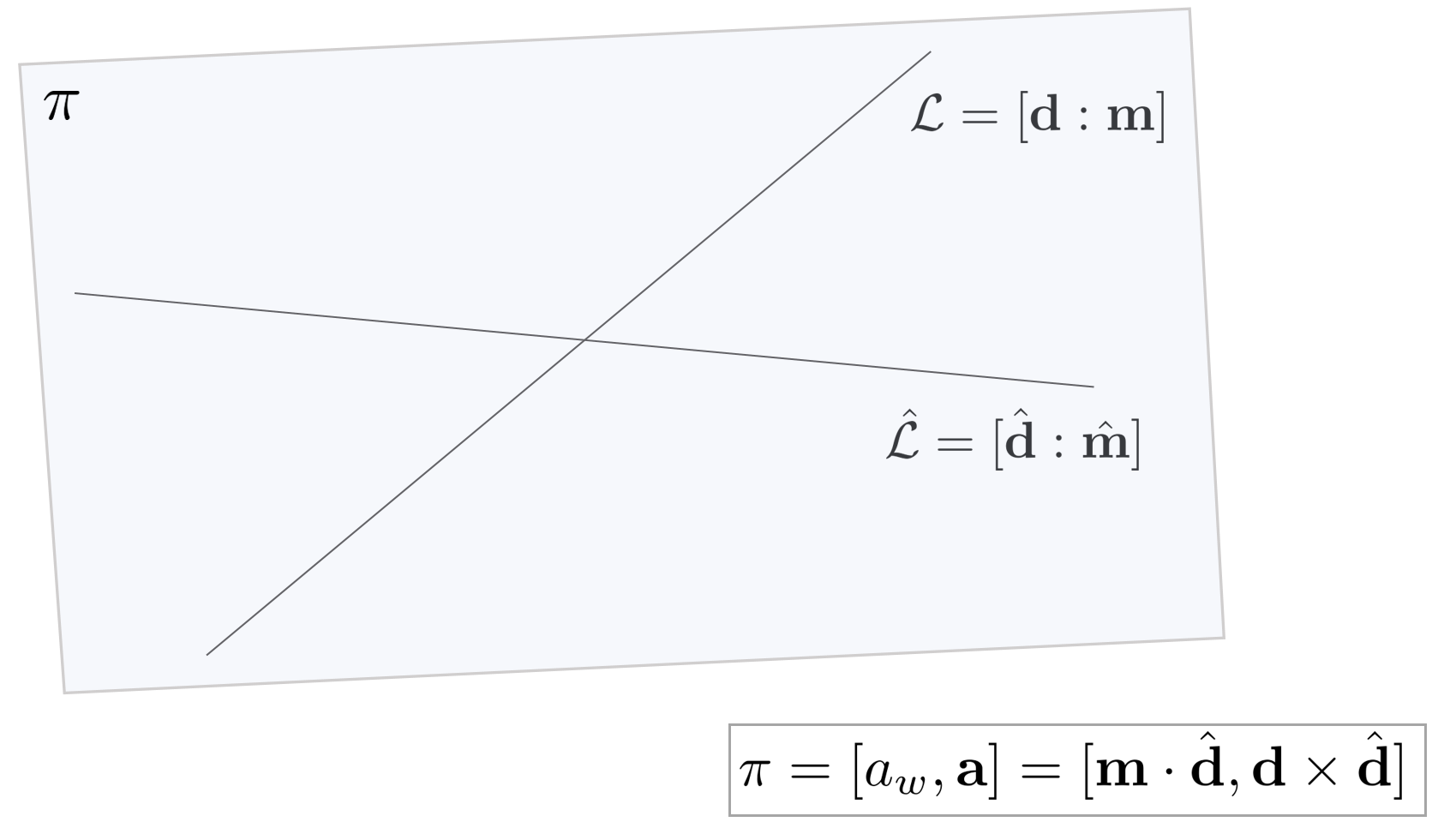
If two lines $\mathcal{L}, \hat{\mathcal{L}}$ in $\mathbb{P}^{3}$ space lie on the same plane $\pi$ (coplanar) and are not parallel to each other, The plane $\pi$ can be obtained through the two lines.
\begin{equation} \begin{aligned}
& \mathcal{L} = [\mathbf{d} : \mathbf{m}] \\
& \hat{\mathcal{L}} = [\hat{\mathbf{d}} : \hat{\mathbf{m}}] \\
& \pi = [a_w, a_x, a_y, a_z] = [a_{w}, \mathbf{a}]
\end{aligned} \end{equation}
The plane $\pi$ can be obtained through the following formula.
\begin{equation} \begin{aligned}
\pi = [a_{w}, \mathbf{a}] = [\mathbf{m} \cdot \hat{\mathbf{d}}, \mathbf{d} \times \hat{\mathbf{d}}]
\end{aligned} \end{equation}
5.3. Line-line meet (Point)

If two lines $\mathcal{L}, \hat{\mathcal{L}}$ in $\mathbb{P}^{3}$ lie on the same plane (coplanar) and are not parallel to each other, then the two lines are They meet at point $\mathbf{X}$.
\begin{equation} \begin{aligned}
& \mathcal{L} = [\mathbf{d} : \mathbf{m}], \quad \\
& \hat{\mathcal{L}} = [\hat{\mathbf{d}} : \hat{\mathbf{m}}] \\
& \mathbf{X} = [W,X,Y,Z] = [W, \tilde{\mathbf{X}}]
\end{aligned} \end{equation}
The 3D point $\mathbf{X}$ can be obtained through the following formula.
\begin{equation} \begin{aligned}
\mathbf{X} = [W, \tilde{\mathbf{X}}] = [\mathbf{d} \cdot \hat{\mathbf{d}}, \mathbf{m} \times \hat{\mathbf{m}}]
\end{aligned} \end{equation}
5.4. Plane-line meet (Point)

A point $\mathbf{X}$ created by the intersection of a line $\mathcal{L}$ and a plane $\pi$ in 3D space is defined as follows.
\begin{equation}
\begin{aligned}
\mathbf{X} = \mathbf{L}\pi
\end{aligned}
\end{equation}
If the line $\mathcal{L}$ exists on the plane $\pi$ then $\mathbf{L}\pi = 0$.
In a little more detail, it is explained as a vector as follows.
\begin{equation} \begin{aligned}
& \mathcal{L} = [\mathbf{d} : \mathbf{m}], \quad \\
& \pi = [a_w, a_x, a_y, a_z] = [a_{w}, \mathbf{a}] \\
& \mathbf{X} = [W,X,Y,Z] = [W, \tilde{\mathbf{X}}]
\end{aligned} \end{equation}
Therefore, a point $\mathbf{X}$ generated by the intersection of a line and a plane is
\begin{equation}
\begin{aligned}
\mathbf{X} = [W, \tilde{\mathbf{X}}] = [\mathbf{a} \cdot \mathbf{d}, \mathbf{a} \times \mathbf{m} - a_{w}\mathbf{d}]
\end{aligned}
\end{equation}
5.5. Point-line join (Plane)

A plane $\pi$ created by a point $\mathbf{X}$ in 3D space and a line $\mathcal{L}$ can be expressed as follows.
\begin{equation}
\begin{aligned}
\pi = \mathbf{L}^{*}\mathbf{X}
\end{aligned}
\end{equation}
If $\mathbf{X}$ exists on the line $\mathcal{L}$ then $\mathbf{L}^{*}\mathbf{X} = 0$. A detailed description of the Dual plücker matrix $\mathbf{L}^{*}$ is explained in the this section.
In a little more detail, it is explained as a vector as follows.
\begin{equation} \begin{aligned}
& \mathcal{L} = [\mathbf{d} : \mathbf{m}], \quad \\
& \mathbf{X} = [W,X,Y,Z] = [W, \tilde{\mathbf{X}}] \\ & \pi = [a_w, a_x, a_y, a_z] = [a_{w}, \mathbf{a}]
\end{aligned} \end{equation}
Therefore, the plane $\pi$ created by a line and a point is
\begin{equation}
\begin{aligned}
\pi = [a_{w}, \mathbf{a}] = [\tilde{\mathbf{X}}\cdot \mathbf{m}, \tilde{\mathbf{X}} \times \mathbf{d} - W\mathbf{m}]
\end{aligned}
\end{equation}
5.6. Line projection to the image plane

Suppose we are given points $\mathbf{A}$ and $\mathbf{B}$ in 3D space and a line $\mathcal{L}$ connecting the two points. Given the camera projection matrix $\mathbf{P}$, the plücker matrix $\mathbf{l}$ of the image of the line $l$ projected on the image plane by the line $\mathcal{L}$ is It can be expressed as:
\begin{equation}
\begin{aligned}
l^{\wedge} = \mathbf{l} = \mathbf{P}\mathbf{L}\mathbf{P}^{\intercal} \in \mathbb{R}^{3\times3}
\end{aligned} \label{eq:5}
\end{equation}
- $\mathcal{L}$: line in 3D space
- $\mathbf{L} = \mathcal{L}^{\wedge}$: plücker matrix of lines in 3D space (skew-symmetric matrix)
- $l$: line projected onto the image plane
- $\mathbf{l} = l^{\wedge}$: plücker matrix of projected lines (skew-symmetric matrix)
5.6.1. Line projection matrix
Using the line projection matrix $\mathcal{P}$, $l$ can be obtained directly without obtaining $\mathbf{l}$ by converting line $\mathcal{L}$ in 3D space to $\mathbf{L}$, which is the form of a plücker matrix, as above. Given an arbitrary camera projection matrix $\mathbf{P} = [\mathbf{N} | \mathbf{n}] \in \mathbb{R}^{3\times 4}$, $\mathcal{P}$ can be defined as follows.
\begin{equation}
\begin{aligned}
\mathcal{P} = [\det(\mathbf{N}) \mathbf{N}^{-\intercal} | \mathbf{n}^{\wedge} \mathbf{N} ] \in \mathbb{R}^{3\times 6}
\end{aligned} \label{eq:6}
\end{equation}
In the case of $\mathbf{P} = [ \mathbf{R} | \mathbf{t} ]$, the above expression can be expressed as follows.
\begin{equation}
\begin{aligned}
\mathcal{P} = [\mathbf{R} \ | \ \mathbf{t}^{\wedge} \mathbf{R} ] \in \mathbb{R}^{3\times 6}
\end{aligned}
\end{equation}
This can be derived through the following equation. Given two points $\mathbf{A}=[\tilde{\mathbf{A}} | a], \mathbf{B} = [\tilde{\mathbf{B}} | b] \in \mathbb{P}^{3}$ in 3D space, suppose there are two points $\mathbf{a}, \mathbf{b} \in \mathbb{P}^{2}$ on the image plane onto which the two points are projected. Through this, the line $l$ can be obtained.
\begin{equation}
\begin{aligned}
l & = \mathbf{a} \times \mathbf{b} \\
& = \mathbf{PA} \times \mathbf{PB} \\
& = (\mathbf{N}\tilde{\mathbf{A}} + a\mathbf{n}) \times (\mathbf{N}\tilde{\mathbf{B}} + b\mathbf{n}) \\
& = (\mathbf{N}\tilde{\mathbf{A}}) \times (\mathbf{N}\tilde{\mathbf{B}}) + a\mathbf{n} \times (\mathbf{N}\tilde{\mathbf{B}}) - b\mathbf{n} \times (\mathbf{N}\tilde{\mathbf{A}}) \\
& = \det(\mathbf{N}) \mathbf{N}^{-\intercal} (\tilde{\mathbf{A}} \times \tilde{\mathbf{B}}) + \mathbf{n}^{\wedge} \mathbf{N}(a \tilde{\mathbf{B}} - b\tilde{\mathbf{A}}) \\
& = [\det(\mathbf{N}) \mathbf{N}^{-\intercal} | \mathbf{n}^{\wedge} \mathbf{N} ] \cdot [ \mathbf{m}^{\intercal} | \mathbf{d}^{\intercal} ]^{\intercal} \\
& = \mathcal{PL}
\end{aligned} \label{eq:7}
\end{equation}
- $\mathbf{m} = \tilde{\mathbf{A}} \times \tilde{\mathbf{B}}$
- $\mathbf{d} = a \tilde{\mathbf{B}} - b\tilde{\mathbf{A}}$
The derivation of the fifth line can be found in the this link.
Alternatively, $\mathcal{P}$ can be obtained. First of all, $\mathcal{P}$ expressed in a different way is as follows.
\begin{equation}
\begin{aligned}
\mathcal{P} = \begin{bmatrix} \mathbf{p}_{2,row} \wedge \mathbf{p}_{3,row} \\ \mathbf{p}_{3,row} \wedge \mathbf{p}_{1,row} \\ \mathbf{p}_{1,row} \wedge \mathbf{p}_{2,row} \end{bmatrix} \in \mathbb{R}^{3\times 6}
\end{aligned}
\end{equation}
- $\mathbf{P} = \begin{bmatrix} \mathbf{p}_{1,row}^{\intercal} \\ \mathbf{p}_{2,row}^{\intercal} \\ \mathbf{p}_{3,row}^{\intercal} \end{bmatrix} \in \mathbb{R}^{3\times 4}$: camera projection matrix
- $\mathbf{p}_{i,row} \in \mathbb{R}^{1\times4}$: $i$th row vector of $\mathbf{P}$. Based on $i=1,2,3$, it means a plane parallel to the $X,Y,Z$ axes, respectively.
- $\mathbf{p}_{i,row} \wedge \mathbf{p}_{j,row} \in \mathbb{R}^{1\times6}$: plücker coordinates of a line resulting from the intersection of two planes $\mathbf{p}_{i,row}$와 $\mathbf{p}_{j,row}$.
Through this, $l$ is obtained as follows.
\begin{equation}
\begin{aligned}
l = \mathcal{P}\mathcal{L} = \begin{bmatrix} ( \mathbf{p}_{2,row} \wedge \mathbf{p}_{3,row} | \mathcal{L} ) \\ ( \mathbf{p}_{3,row} \wedge \mathbf{p}_{1,row} | \mathcal{L} ) \\ ( \mathbf{p}_{1,row} \wedge \mathbf{p}_{2,row} | \mathcal{L} ) \end{bmatrix}
\end{aligned}
\end{equation}
Since the $\mathbf{a}, \mathbf{b}$ projected by two points $\mathbf{A}, \mathbf{B}$ in the 3D space can be expressed as $\mathbf{a} = \mathbf{PA}, \mathbf{b} = \mathbf{PB}$ and as the image $l = \mathbf{a} \times \mathbf{b} = (\mathbf{PA} \times \mathbf{PB})$ of a line, it can be developed as follows according to (\ref{eq:1}).
\begin{equation}
\begin{aligned}
l & = \mathbf{PA} \times \mathbf{PB} \\
& = \bigg( \begin{bmatrix} \mathbf{p}_{1,row} \\ \mathbf{p}_{2,row} \\ \mathbf{p}_{3,row} \end{bmatrix} \mathbf{A} \bigg) \times \bigg( \begin{bmatrix} \mathbf{p}_{1,row} \\ \mathbf{p}_{2,row} \\ \mathbf{p}_{3,row} \end{bmatrix} \mathbf{B} \bigg) \\
& = \begin{bmatrix} \mathbf{p}_{1,row}\mathbf{A} \\ \mathbf{p}_{2,row}\mathbf{A} \\ \mathbf{p}_{3,row}\mathbf{A} \end{bmatrix} \times \begin{bmatrix} \mathbf{p}_{1,row}\mathbf{B} \\ \mathbf{p}_{2,row}\mathbf{B} \\ \mathbf{p}_{3,row}\mathbf{B} \end{bmatrix} \\
& = \begin{bmatrix} 0 & -\mathbf{p}_{3,row}\mathbf{A} & \mathbf{p}_{2,row}\mathbf{A} \\ \mathbf{p}_{3,row}\mathbf{A} & 0 & -\mathbf{p}_{1,row}\mathbf{A} \\ -\mathbf{p}_{2,row}\mathbf{A} & \mathbf{p}_{1,row}\mathbf{A} & 0 \end{bmatrix} \begin{bmatrix} \mathbf{p}_{1,row}\mathbf{B} \\ \mathbf{p}_{2,row}\mathbf{B} \\ \mathbf{p}_{3,row}\mathbf{B} \end{bmatrix} \\
& = \begin{bmatrix} (\mathbf{p}_{2,row}^{\intercal}\mathbf{A})(\mathbf{p}_{3,row}^{\intercal}\mathbf{B}) - (\mathbf{p}_{2,row}^{\intercal}\mathbf{B}) (\mathbf{p}_{3,row}^{\intercal}\mathbf{A}) \\ (\mathbf{p}_{3,row}^{\intercal}\mathbf{A})(\mathbf{p}_{1,row}^{\intercal}\mathbf{B}) - (\mathbf{p}_{3,row}^{\intercal}\mathbf{B}) (\mathbf{p}_{1,row}^{\intercal}\mathbf{A}) \\ (\mathbf{p}_{1,row}^{\intercal}\mathbf{A})(\mathbf{p}_{2,row}^{\intercal}\mathbf{B}) - (\mathbf{p}_{1,row}^{\intercal}\mathbf{B}) (\mathbf{p}_{2,row}^{\intercal}\mathbf{A}) \end{bmatrix} && \\
& = \begin{bmatrix} (\mathbf{p}_{2,row} \wedge \mathbf{p}_{3,row} | \mathcal{L}) \\ (\mathbf{p}_{3,row} \wedge \mathbf{p}_{1,row} | \mathcal{L}) \\ (\mathbf{p}_{1,row} \wedge \mathbf{p}_{2,row} | \mathcal{L}) \end{bmatrix} && \cdots \text{ by } (\ref{eq:1})
\end{aligned}
\end{equation}

Each row vector of the $\mathcal{P}$ matrix represents a line geometrically, similar to how each row vector of the $\mathbf{P}$ matrix represents a plane. If the $\mathbf{p}_{i,row}$ matrix means the X,Y axis plane and the principal plane, then the row vector of the $\mathcal{P}$ matrix means the intersection of the planes. In other words, the row vector of $\mathcal{P}$ means a line passing through the camera's center point $\tilde{\mathbf{C}}$ and parallel to each $X,Y,Z$.
For example, the first row vector of $\mathcal{P}$ is $[\mathbf{p}_{2,row} \wedge \mathbf{p}_{3,row}]$, which is $y=0$ It means a line where the plane $\mathbf{p}_{2,row}$ and the main plane $\mathbf{p}_{3,row}$ intersect each other. If $\mathcal{PL} = 0$ for a line $\mathcal{L}$ in 3D space, it means that the corresponding line exists in the null space of $\mathcal{P}$. This means $\mathcal{L}$ passes through the camera center point $\tilde{\mathbf{C}}$.
5.6.2. Point and line duality

Previously, it was said that the skew-symmetric matrix of the line $l$ projected by the line $\mathcal{L}$ in the 3D space can be obtained through $\mathbf{l} = \mathbf{PLP}^{\intercal}$ of the (\ref{eq:5}). This can also be expressed as:
\begin{equation}
\begin{aligned}
l^{\wedge} & = (\mathbf{a} \times \mathbf{b})^{\wedge} \\
& = \mathbf{ab}^{\intercal} - \mathbf{ba}^{\intercal} = \begin{bmatrix} 0&l_2&-l_{1} \\ -l_{2} & 0 & l_{0} \\ l_{1} & -l_{0} & 0 \end{bmatrix} \\
& = \mathbf{l}
\end{aligned}
\end{equation}
- $l \in \mathbb{R}^{3}$: a line on the image
- $l^{\wedge} \in \mathbb{R}^{3\times3}$: skew-symmetric matrix of line $l$
- $\mathbf{a}, \mathbf{b}$: Projected points of $\mathbf{A}, \mathbf{B}$ in 3D space
By the property of the cross product, when it is $\mathbf{a} = \mathbf{b} \times \mathbf{c}$, it becomes $\mathbf{a}^{\wedge} = \mathbf{bc}^{\intercal} - \mathbf{cb}^{\intercal}$.
Duality: The intersection $\mathbf{a}$ of two lines $l, m$ projected by two lines $\mathcal{L}, \mathcal{M}$ in 3D space can be expressed as follows.
\begin{equation}
\begin{aligned}
\mathbf{a}^{\wedge} = lm^{\intercal} - ml^{\intercal} \in \mathbb{R}^{3\times3}
\end{aligned}
\end{equation}
- $\mathbf{a}^{\wedge}$: skew symmetric matrix of $\mathbf{a}$
5.6.3. Projection matrix duality
Next, the projection matrix also has duality.

The line projection matrix $\mathcal{P}$ performs the same function as the three-dimensional point projection matrix $\mathbf{P}$.
\begin{equation}
\begin{aligned}
\mathbf{x} & = \mathbf{PX} \\ l & = \mathcal{P}\mathcal{L}
\end{aligned}
\end{equation}
6. Plücker line-based optimization

A line in 3D space can be expressed as a 6D column vector using Plücker coordinates.
\begin{equation}
\begin{aligned}
\mathcal{L} & = [\mathbf{m}^{\intercal} : \mathbf{d}^{\intercal}]^{\intercal} = [ m_{x} : m_{y} : m_{z} : d_{x} : d_{y} : d_{z}]^{\intercal}
\end{aligned}
\end{equation}
Unlike the $[\mathbf{d} : \mathbf{m}]$ order described above, most papers using Plücker Coordinate use the $[\mathbf{m} : \mathbf{d}]$ order, so this section Also, lines are expressed in the corresponding order. Since the linear expression method has scale ambiguity, it has 5 degrees of freedom, and even if $\mathbf{m}$ and $\mathbf{d}$ are not unit vectors, a line can be uniquely expressed by the ratio of the values of the two vectors.
6.1. Line Transformation and projection
If $\mathcal{L}_{w}$ is the line viewed from the world coordinate system, it can be converted as follows when viewed from the camera coordinate system.[8].
\begin{equation}
\begin{aligned}
\mathcal{L}_{c} & = \begin{bmatrix} \mathbf{m}_{c} \\ \mathbf{d}_{c} \end{bmatrix} = \mathcal{T}_{cw}\mathcal{L}_{w} = \begin{bmatrix} \mathbf{R}_{cw} & \mathbf{t}^{\wedge}\mathbf{R}_{cw} \\ 0 & \mathbf{R}_{cw} \end{bmatrix} \begin{bmatrix} \mathbf{m}_{w} \\ \mathbf{d}_{w} \end{bmatrix}
\end{aligned}
\end{equation}
- $\mathcal{T}_{cw} \in \mathbb{R}^{6\times6}$: transformation matrix of Plücker line
Projecting the line onto the image plane gives:
\begin{equation}
\begin{aligned}
l_{c} & = \begin{bmatrix} l_{1} \\ l_{2} \\ l_{3} \end{bmatrix} = \mathcal{K}_{L}\mathbf{m}_{c} = \begin{bmatrix} f_{y} && \\ &f_{x} & \\ -f_{y}c_{x} & -f_{x}c_{y} & f_{x}f_{y} \end{bmatrix} \begin{bmatrix} m_{x} \\ m_{y} \\ m_{z} \end{bmatrix}
\end{aligned}
\end{equation}
- $\mathcal{K}_{L}$: line intrinsic matrix
$\mathcal{K}_{L}$ means $\mathcal{P} = [\det(\mathbf{N}) \mathbf{N}^{-\intercal} | \mathbf{n}^{\wedge} \mathbf{N} ]$ to $\mathbf{P} = K [ \mathbf{I} | \mathbf{0}]$. So $\mathcal{P} = [\det(\mathbf{K})\mathbf{K}^{-\intercal} | \mathbf{0}]$, so the $\mathbf{d}$ term of $\mathcal{L}$ is cleared to 0. Therefore, when $\mathbf{K} = \begin{bmatrix} f_x & & c_x \\ & f_y & c_y \\ &&1 \end{bmatrix}$, the following expression is derived.
\begin{equation}
\begin{aligned}
\mathcal{K}_{L} = \det(\mathbf{K})\mathbf{K}^{-\intercal} = \begin{bmatrix} f_{y} && \\ &f_{x} & \\ -f_{y}c_{x} & -f_{x}c_{y} & f_{x}f_{y} \end{bmatrix} \in \mathbb{R}^{3\times3}
\end{aligned}
\end{equation}
6.2. Line reprojection error

The reprojection error $\mathbf{e}_{l}$ of a line can be expressed as follows.
\begin{equation}
\begin{aligned}
\mathbf{e}_{l} = \begin{bmatrix} d_{s}, \ d_{e} \end{bmatrix}= \begin{bmatrix} \frac{\mathbf{x}_{s}^{\intercal}l_{c}}{\sqrt{l_{1}^{2} + l_{2}^{2}}}, & \frac{\mathbf{x}_{e}^{\intercal}l_{c}}{\sqrt{l_{1}^{2} + l_{2}^{2}}}\end{bmatrix} \in \mathbb{R}^{2}
\end{aligned}
\end{equation}
This can be expressed through the formula for the distance between a point and a line. At this time, $\{\mathbf{x}_{s}$ and $\mathbf{x}_{e}\}$ mean the start and end points of the line extracted using line feature extracture (e.g., LSD), respectively.
6.3. Orthonormal representation
A problem arises if the Plücker Coordinate expression is used as it is when BA optimization is performed using $\mathbf{e}_{l}$ obtained above. Since the Plücker Coordinate always has 5 degrees of freedom because it must satisfy the Klein quadric constraint of $\mathbf{m}^{\intercal}\mathbf{d} = 0$, the minimum number of parameters that can express a line is 4 It is over-parameterized. Disadvantages of over-parameterized representation are as follows[6]:
- Since overlapping parameters must be calculated, the amount of computation increases during optimization.
- Additional degrees of freedom may cause numerical instability problems.
- Whenever a parameter is updated, it must always be checked whether the constraint is satisfied.
Therefore, when optimizing a line, an orthonormal expression is usually used to change the minimum parameter to four degrees of freedom[4][5][6][7]. In other words, when expressing a line, Plücker Coordinate is used, but when performing optimization, it transforms into orthonormal expression, updates the optimal value, and returns to Plücker Coordinate.
Orthonormal expression is as follows. A line in 3D space can always be expressed as[6].
\begin{equation}
\begin{aligned}
(\mathbf{U}, \mathbf{W}) \in SO(3) \times SO(2)
\end{aligned}
\end{equation}
- $\mathbf{U} \in SO(3)$: rotation matrix of a three-dimensional line
- $\mathbf{W} \in SO(2)$: A matrix containing information on the distance a 3D line is from the origin
Any Plücker line $\mathcal{L} = [\mathbf{m}^{\intercal} : \mathbf{d}^{\intercal}]^{\intercal}$ always has a one-to-one correspondence $(\mathbf{U}, \mathbf{W})$, and this representation method is called orthonormal representation. Given a line $\mathcal{L}_{w} = [ \mathbf{m}_{w}^{\intercal} : \mathbf{d}_{w}^{\intercal}]^{\intercal}$ in the world, $(\mathbf{U}, \mathbf{W})$ can be obtained by performing QR decomposition of $\mathcal{L}_{w}$.
\begin{equation}
\begin{aligned}
\begin{bmatrix} \mathbf{m}_{w} \ | \ \mathbf{d}_{w} \end{bmatrix}= \mathbf{U} \begin{bmatrix} w_{1} & 0\\ 0& w_{2} \\0 & 0 \end{bmatrix}, \quad \text{with set: } \mathbf{W} = \begin{bmatrix} w_{1} & -w_{2} \\ w_{2} & w_{1} \end{bmatrix}
\end{aligned}
\end{equation}
At this time, the element $(1,2)$ of the upper triangle matrix $\mathbf{R}$ always becomes 0 due to the Plücker constraint (Klein quadric). Since $\mathbf{U}$ and $\mathbf{W}$ mean 3D and 2D rotation matrices, respectively, $\mathbf{U} = \mathbf{R}(\boldsymbol{\theta}), \mathbf{W } = \mathbf{R}(\theta)$.
\begin{equation}
\begin{aligned}
\mathbf{R}(\boldsymbol{\theta}) & = \mathbf{U} = \begin{bmatrix} \mathbf{u}_{1} & \mathbf{u}_{2} & \mathbf{u}_{3} \end{bmatrix} = \begin{bmatrix} \frac{\mathbf{m}_{w}}{\left\| \mathbf{m}_{w} \right\|} & \frac{\mathbf{d}_{w}}{\left\| \mathbf{d}_{w} \right\|} & \frac{\mathbf{m}_{w} \times \mathbf{d}_{w}}{\left\| \mathbf{m}_{w} \times \mathbf{d}_{w} \right\|} \end{bmatrix} \\
\mathbf{R}(\theta) & = \mathbf{W} = \begin{bmatrix} w_{1} & -w_{2} \\ w_{2} & w_{1} \end{bmatrix} = \begin{bmatrix} \cos\theta & -\sin\theta \\ \sin\theta & \cos\theta \end{bmatrix} \\
& = \frac{1}{\sqrt{\left\| \mathbf{m}_{w} \right\|^{2} + \left\| \mathbf{d}_{w} \right\|^{2}}} \begin{bmatrix} \left\| \mathbf{m}_{w} \right\| & \left\| \mathbf{d}_{w} \right\| \\ -\left\| \mathbf{d}_{w} \right\| & \left\| \mathbf{m}_{w} \right\| \end{bmatrix}
\end{aligned}
\end{equation}
- $\boldsymbol{\theta} \in \mathbb{R}^{3}$: parameter corresponding to SO(3) rotation matrix
- $\theta \in \mathbb{R}$: parameter corresponding to SO(2) rotation matrix
- $\mathbf{u}_{i}$: $i$th column vector
When performing real optimizations, they are updated like $\mathbf{U} \leftarrow \mathbf{U}\mathbf{R}(\boldsymbol{\theta}), \mathbf{W} \leftarrow \mathbf{W}\mathbf{R}(\theta)$. So the orthonormal representation is a line in 3D space $\delta_{\boldsymbol{\theta}} = [ \boldsymbol{\theta}^{\intercal}, \theta ] \in \mathbb{R}^{4}$ can be expressed with four degrees of freedom. $[ \boldsymbol{\theta}^{\intercal}, \theta ]$ updated through optimization is converted to $\mathcal{L}_{w}$ as follows.
\begin{equation}
\begin{aligned}
\mathcal{L}_{w} = \begin{bmatrix} w_{1} \mathbf{u}_{1}^{\intercal} & w_{2} \mathbf{u}_{2}^{\intercal} \end{bmatrix}
\end{aligned}
\end{equation}
6.4. Error function formulation
In order to optimize the reprojection error $\mathbf{e}_{l}$ for a line, iteratively using a nonlinear least squares method such as Gauss-Newton (GN) or Levenberg-Marquardt (LM) to find the optimal variable. need to update The expression of the error function using the reprojection error is as follows.
\begin{equation}
\begin{aligned}
\mathbf{E}_{l}(\mathcal{X}) & = \arg\min_{\mathcal{X}^{*}} \sum_{i}\sum_{j} \left\| \mathbf{e}_{l,ij} \right\|^{2} \\
& = \arg\min_{\mathcal{X}^{*}} \sum_{i}\sum_{j} \mathbf{e}_{l,ij}^{\intercal}\mathbf{e}_{l,ij} \\
\end{aligned} \label{eq:10}
\end{equation}
- $\mathcal{X} = [\delta_{\boldsymbol{\theta}}, \delta_\xi ]$: state variable
- $\delta_{\boldsymbol{\theta}} = [ \boldsymbol{\theta}^{\intercal}, \theta ] \in \mathbb{R}^{4}$: state variable in orthonormal representation
- $\delta_{\xi} = [\delta \xi] \in se(3)$: Refer to this link for an update method through Lie theory
The $\left\|\mathbf{e}_{l}(\mathcal{X}^{*})\right\|^{2}$ satisfying $\mathbf{E}_{l}(\mathcal{X}^{*})$ can be calculated iteratively through non-linear least squares. The optimal state is found by iteratively updating $\mathcal{X}$ in small increments $\Delta \mathcal{X}$.
\begin{equation}
\begin{aligned}
\mathbf{E}_{l}(\mathcal{X} + \Delta \mathcal{X}) & = \arg\min_{\mathcal{X}^{*}} \sum_{i}\sum_{j} \left\|\mathbf{e}_{l}(\mathcal{X} +\Delta \mathcal{X})\right\|^{2}
\end{aligned}
\end{equation}
Strictly speaking, since the state increment $\Delta \mathcal{X}$ includes the SE(3) transformation matrix, it is correct to add it to the existing state $\mathcal{X}$ through the $\oplus$ operator, but for convenience of expression The $+$ operator is used.
\begin{equation}
\begin{aligned}
\mathbf{e}_{l}( \mathcal{X} \oplus \Delta \mathcal{X})
\quad \rightarrow \quad\mathbf{e}_{l}(\mathcal{X} + \Delta \mathcal{X})
\end{aligned}
\end{equation}
- $\oplus$ : An operator that can update state variables $\delta{\boldsymbol{\theta}}$ and $\delta\xi$ at once.
The above equation can be expressed as follows through Taylor's first-order approximation.
\begin{equation}
\begin{aligned}
\mathbf{e}_{l}(\mathcal{X} + \Delta \mathcal{X}) & \approx \mathbf{e}_{l}(\mathcal{X}) + \mathbf{J}\Delta \mathcal{X} \\ & = \mathbf{e}_{l}(\mathcal{X}) + \mathbf{J}_{\boldsymbol{\theta}} \Delta \delta_{\boldsymbol{\theta}} +\mathbf{J}_{\xi} \Delta \delta_\xi \\
& = \mathbf{e}_{l}(\mathcal{X}) + \frac{\partial \mathbf{e}_{l}}{\partial \delta_{\boldsymbol{\theta}}} \Delta \delta_{\boldsymbol{\theta}} + \frac{\partial \mathbf{e}_{l}}{\partial \delta_\xi}\Delta \delta_\xi \\
\end{aligned}
\end{equation}
- $\mathbf{J} = \frac{\partial \mathbf{e}_{l}}{\partial \mathcal{X}} = \frac{\partial \mathbf{e}_{l}}{\partial [\delta_{\boldsymbol{\theta}}, \delta_\xi]}$
\begin{equation}
\begin{aligned}
\mathbf{E}_{l}(\mathcal{X} + \Delta \mathcal{X}) & \approx \arg\min_{\mathcal{X}^{*}} \sum_{i}\sum_{j} \left\|\mathbf{e}_{l}(\mathcal{X}) + \mathbf{J}\Delta \mathcal{X} \right\|^{2} \\
\end{aligned}
\end{equation}
By differentiating this, the optimal value of increment $\Delta \mathcal{X}^{*}$ is obtained as follows. The detailed derivation process is omitted in this document. If you want to know more about the induction process, please refer to this link.
\begin{equation}
\begin{aligned}
& \mathbf{J}^{\intercal}\mathbf{J} \Delta \mathcal{X}^{*} = -\mathbf{J}^{\intercal}\mathbf{e} \\
& \mathbf{H}\Delta \mathcal{X}^{*} = - \mathbf{b} \\
\end{aligned}
\end{equation}
6.4.1. The analytical jacobian of 3d line
As explained in the previous section, to perform nonlinear optimization we need to compute $\mathbf{J}$. $\mathbf{J}$ consists of:
\begin{equation}
\begin{aligned}
& \mathbf{J} = [ \mathbf{J}_{\boldsymbol{\theta}}, \mathbf{J}_{\xi} ]
\end{aligned}
\end{equation}
$[ \mathbf{J}_{\boldsymbol{\theta}}, \mathbf{J}_{\xi} ]$ can be expanded as follows:
\begin{equation}
\begin{aligned}
& \mathbf{J}_{\boldsymbol{\theta}} = \frac{\partial \mathbf{e}_{l}}{\partial \delta_{\boldsymbol{\theta}}} = \frac{\partial \mathbf{e}_{l}}{\partial l} \frac{\partial l}{\partial \mathcal{L}_{c}} \frac{\partial \mathcal{L}_{c}}{\partial \mathcal{L}_{w}} \frac{\partial \mathcal{L}_{w}}{\partial \delta_{\boldsymbol{\theta}}} \\
& \mathbf{J}_{\xi} = \frac{\partial \mathbf{e}_{l}}{\partial \delta_{\xi}} = \frac{\partial \mathbf{e}_{l}}{\partial l} \frac{\partial l}{\partial \mathcal{L}_{c}} \frac{\partial \mathcal{L}_{c}}{\partial \delta_{\xi}}
\end{aligned}
\end{equation}
$\frac{\partial \mathbf{e}_{l}}{\partial l}$ can be obtained as follows. At this time, note that $l$ is a vector and $l_{i}$ is a scalar.
\begin{equation}
\begin{aligned}
\frac{\partial \mathbf{e}_{l}}{\partial l} = \frac{1}{\sqrt{l_{1}^{2} + l_{2}^{2}}} \begin{bmatrix} x_{s} - \frac{l_{1} \mathbf{x}_{s}l}{\sqrt{l_{1}^{2} + l_{2}^{2}}} & y_{s} - \frac{l_{2} \mathbf{x}_{s}l}{\sqrt{l_{1}^{2} + l_{2}^{2}}} & 1 \\
x_{e} - \frac{l_{1} \mathbf{x}_{e}l}{\sqrt{l_{1}^{2} + l_{2}^{2}}} & y_{e} - \frac{l_{2} \mathbf{x}_{e}l}{\sqrt{l_{1}^{2} + l_{2}^{2}}} & 1 \end{bmatrix} \in \mathbb{R}^{2\times3}
\end{aligned}
\end{equation}
$\frac{\partial l}{\partial \mathcal{L}_{c}}$ can be obtained as follows.
\begin{equation}
\begin{aligned}
\frac{\partial l}{\partial \mathcal{L}_{c}} = \frac{\partial \mathcal{K}_{L}\mathbf{m}_{c}}{\partial \mathcal{L}_{c}} = \begin{bmatrix} \mathcal{K}_{L} & \mathbf{0}_{3\times3} \end{bmatrix} = \begin{bmatrix} f_{y} && & 0 &0&0 \\ &f_{x} & & 0 &0&0 \\ -f_{y}c_{x} & -f_{x}c_{y} & f_{x}f_{y} & 0 &0&0 \end{bmatrix} \in \mathbb{R}^{3\times6}
\end{aligned}
\end{equation}
$\frac{\partial \mathcal{L}_{c}}{\partial \mathcal{L}_{w}}$ can be obtained as follows.
\begin{equation}
\begin{aligned}
\frac{\partial \mathcal{L}_{c}}{\partial \mathcal{L}_{w}} = \frac{\partial \mathcal{T}_{cw}\mathcal{L}_{w}}{\partial \mathcal{L}_{w}}= \mathcal{T}_{cw} = \begin{bmatrix} \mathbf{R}_{cw} & \mathbf{t}^{\wedge}\mathbf{R}_{cw} \\ 0 & \mathbf{R}_{cw} \end{bmatrix} \in \mathbb{R}^{6\times6}
\end{aligned}
\end{equation}
The Jacobian $\frac{\partial \mathcal{L}_{w}}{\partial \delta_{\boldsymbol{\theta}}}$ for the orthonormal representation can be obtained as [8].
\begin{equation}
\begin{aligned}
\frac{\partial \mathcal{L}_{w}}{\partial \delta_{\boldsymbol{\theta}}} = \begin{bmatrix} \mathbf{0}_{3\times1} & -w_{1}\mathbf{u}_{3} & w_{1}\mathbf{u}_{2} & -w_{2}\mathbf{u}_{1} \\ w_{2}\mathbf{u}_{3} & \mathbf{0}_{3\times1} & -w_{2}\mathbf{u}_{1} & w_{1}\mathbf{u}_{2} \end{bmatrix} \in \mathbb{R}^{6 \times 4}
\end{aligned}
\end{equation}
The Jacobian $\frac{\partial \mathcal{L}_{c}}{\partial \delta_{\xi}}$ for the camera pose can be obtained as [9].
\begin{equation}
\begin{aligned}
\frac{\partial \mathcal{L}_{c}}{\partial \delta_{\xi}} = \begin{bmatrix} -(\mathbf{R}\mathbf{m})^{\wedge} - (\mathbf{t}^{\wedge} \mathbf{Rd})^{\wedge} & -(\mathbf{Rd})^{\wedge} \\ -(\mathbf{Rd})^{\wedge} & \mathbf{0}_{3\times3} \end{bmatrix} \in \mathbb{R}^{6 \times 6}
\end{aligned}
\end{equation}
7. References
[3] [Wiki] Plücker Coordinates
8. Closure
The pdf version is available soon.
'English' 카테고리의 다른 글
| [SLAM][En] Direct Sparse Odometry (DSO) Paper Review Part 1 (0) | 2023.01.17 |
|---|---|
| [En] Notes on Lie Theory (SO(3), SE(3)) (0) | 2023.01.17 |
| [SLAM][En] Errors and Jacobian Derivations for SLAM Part 2 (0) | 2023.01.17 |
| [SLAM][En] Errors and Jacobian Derivations for SLAM Part 1 (0) | 2023.01.17 |
| [En] Vim - Useful plugins and C++/Python development environment (1) | 2023.01.16 |


