추정 이론(Estimation Theory) 개념 정리 Part 2 - RBLS, BLUE, MLE, LSE, Exponential Familiy

5. General Minimum Variance Unbiased Estimation

이전 섹션에서 CRLB를 통해 추정값이 efficient함을 알 수 있고 efficient한 추정값은 MVUE가 되는 것을 알 수 있었다. 그리고 선형 모델(linear model)을 사용하여 다양한 예제를 확인하였다. 하지만 만약 efficient한 추정값이 존재하지 않더라도 MVUE를 찾는 것에 관심이 있을 수 있다. 이번 섹션에서는 이러한 관심사를 확인할 수 있는 Rao-Blackwell-Lehmann-Scheffe(RBLS) 이론에 대해 배우고 이를 위한 충분통계량(sufficient statistics)의 개념에 대해 배운다. RBLS를 사용하면 많은 경우 단순히 pdf를 보는 것 만으로도 MVUE 인지 여부를 판단할 수 있게 된다.

5.1. Sufficient Statistics

이전 챕터에서 DC Level $A$의 추정 문제를 다시 보면 다음과 같다.

\begin{equation} \label{eq:ss1}
\begin{aligned}
x[n] =  A + w[n]
\end{aligned}
\end{equation}

- $w[n] \sim \mathcal{N}(0, \sigma^2)$ : WGN

$A$의 추정값 $\hat{A}$는 다음과 같이 데이터의 평균으로 구하였다.

\begin{equation}
\begin{aligned}
\hat{A} = \frac{1}{N} \sum_{n=0}^{N-1} x[n]
\end{aligned}
\end{equation}

$\hat{A}$는 MVUE이므로 최소 분산 $\frac{\sigma^2}{N}$을 가진다. 만약 다음과 같은 추정값을 사용한다고 가정하자.

\begin{equation}
\begin{aligned}
\breve{A} = x[0]
\end{aligned}
\end{equation}

$\breve{A}$는 편향되지 않았다는 것(unbiased)을 알 수 있지만 $\breve{A}$의 분산은 $\sigma^{2}$로 MVUE의 분산$\frac{\sigma^2}{N}$ 대비 크다는 것을 알 수 있다. 직관적으로 다른 데이터 $x[1], x[2], \cdots, x[N-1]$을 사용하지 않기 때문에 $A$에 대한 정보를 상실하여 좋은 추정값이 아님을 알 수 있다. 여기서 어떤 데이터가 $A$의 정보를 많이 포함하고 있을까? 또는 어떤 데이터가 $A$를 추정하는데 충분할까? 아래와 같이 추정에 사용 가능한 집합들이 주어졌다고 가정해보자.

\begin{equation}
\begin{aligned}
& S_1 = \{ x[0], x[1], \cdots, x[N-1] \} \\
& S_2 = \{x[0]+x[1], x[2], x[3], \cdots, x[N-1] \} \\
& S_3 = \{ \sum_{n=0}^{N-1} x[n] \}
\end{aligned}
\end{equation}

$S_1$은 기존 데이터 집합으로써 항상 충분한 데이터를 가지고 있다. $S_2$와 $S_3$ 또한 충분한 데이터를 가지고 있다. 이외에도 예제를 만족하는 수 많은 충분한 데이터 집합들이 있지만 우리는 이 중 가장 최소한의 크기를 지닌 집합을 원한다. $S_1, S_2, S_3$ 모두 통계적 관점에서 sufficient하다고 볼 수 있지만 이 중 가장 작은 크기의 집합인 $S_3$는 특별히 minimal sufficient statistics(또는 충분통계량)라고 한다. $A$를 추정할 때 $\sum_{n=0}^{N-1} x[n]$은 각 데이터에 대한 모든 정보를 포함하고 있으므로 개별 데이터를 알지 못해도 추정이 가능하다.

충분통계량을 자세히 알기 위해 pdf를 보면 다음과 같다.

\begin{equation} \begin{aligned}
p(\mathbf{x};A) = \frac{1}{ (2\pi\sigma^{2})^{\frac{N}{2}} } \exp\bigg[ -\frac{1}{2\sigma^{2}} \sum_{n=0}^{N-1}(x[n] - A)^{2} \bigg]
\end{aligned} \end{equation}

위 식에 임의의 통계량을 $T(\mathbf{x}) = \sum_{n=0}^{N-1} x[n]$이 주어진 경우 pdf $p(\mathbf{x} | T(\mathbf{x}) ; A)$가 파라미터 $A$에 더 이상 종속적이지 않다면 $T(\mathbf{x})$는 파라미터를 추정하는데 충분한 통계량(i.e., 충분통계량)이라고 정의한다.

5.1.1. Example 5.1 - Verification of a Sufficient Statistic

(\ref{eq:ss1})를 사용하여 충분통계량이 $A$에 독립적임을 증명해보자. 통계량 $T(\mathbf{x})=T_0$이 주어진 경우 조건부 pdf는 다음과 같이 전개할 수 있다.

\begin{equation} \begin{aligned}
p(\mathbf{x}|T(\mathbf{x})=T_0;A) = \frac{p(\mathbf{x}, T(\mathbf{x})=T_0;A)}{p(T(\mathbf{x})=T_0;A)}
\end{aligned} \end{equation}

- $T( \mathbf{x}) = \sum_{n=0}^{N-1}x[n]$

위 식의 우측 상단의 joint pdf는 다음과 같이 Dirac delta function을 사용하여 분리할 수 있다. (자세한 내용은 Appendix 5A 참조)

\begin{equation} \label{eq:ss2} \begin{aligned}
p(\mathbf{x}|T(\mathbf{x})=T_0;A) = \frac{p(\mathbf{x};A) \delta( T(\mathbf{x})-T_0)}{p(T(\mathbf{x})=T_0;A)}
\end{aligned} \end{equation}

통계량은 정의 상 $T( \mathbf{x}) \sim \mathcal{N}(NA, N\sigma^2)$을 만족하므로 위 식은 다음과 같이 전개할 수 있다.

\begin{equation} \label{eq:ss3} \begin{aligned}
p(\mathbf{x};A) \delta( T(\mathbf{x})-T_0) & = \frac{1}{(2\pi \sigma^2)^{\frac{N}{2}}} \exp\bigg[ -\frac{1}{2\sigma^2} \sum_{n=0}^{N-1}(x[n]-A)^{2} \bigg] \delta (T(\mathbf{x}) - T_0) \\
& = \frac{1}{(2\pi \sigma^2)^{\frac{N}{2}}} \exp\bigg[ -\frac{1}{2\sigma^2} \bigg( \sum_{n=0}^{N-1} {\color{Cyan} x^2[n] - 2AT(\mathbf{x}) + NA^2 } \bigg) \bigg] \delta (T(\mathbf{x}) - T_0) \\
& = \frac{1}{(2\pi \sigma^2)^{\frac{N}{2}}} \exp\bigg[ -\frac{1}{2\sigma^2} \bigg( \sum_{n=0}^{N-1} x^2[n] - 2A {\color{Cyan} T_0 } + NA^2 \bigg) \bigg] \delta (T(\mathbf{x}) - T_0) \\
\end{aligned} \end{equation}

(\ref{eq:ss3})을 (\ref{eq:ss2})에 대입하면 다음과 같다.

\begin{equation} \begin{aligned}
p(\mathbf{x}|T(\mathbf{x})=T_0;A) & = \frac{ \frac{1}{(2\pi \sigma^2)^{\frac{N}{2}}} \exp\bigg[ -\frac{1}{2\sigma^2}\sum_{n=0}^{N-1}x^2[n] \bigg] \exp \bigg[ -\frac{1}{2\sigma^2}(-2AT_0 +NA^2) \bigg] }{ \frac{1}{\sqrt{2\pi N\sigma^2}} \exp\bigg[ -\frac{1}{2N\sigma^2} (T_0 - NA)^2 \bigg] } \delta (T(\mathbf{x}) - T_0) \\
& = \frac{\sqrt{N}}{ (2\pi\sigma^2)^{\frac{N-1}{2}} } \exp\bigg[ -\frac{1}{2\sigma^2} \sum_{n=0}^{N-1}x^2[n] \bigg] \exp \bigg[ \frac{T_0^2}{2N\sigma^2} \bigg] \delta (T(\mathbf{x}) - T_0)
\end{aligned} \end{equation}

위 식 마지막 줄에서 보다시피 파라미터 $A$가 존재하지 않으므로 더 이상 $A$에 종속적이지 않다. 따라서 $T( \mathbf{x}) = \sum_{n=0}^{N-1}x[n]$는 $A$를 추정하는데 충분한 통계량(i.e., 충분통계량)인 것을 알 수 있다.

5.2. Finding Sufficient Statistics

5.2.1. Theorem 5.1 (Neyman-Fisher Factorization)

임의의 통계량 $T(\mathbf{x})$이 파라미터 $\theta$에 대한 충분통계량이면 $p(\mathbf{x};\theta)$는 반드시 다음과 같은 형태로 분해(factorization)할 수 있다. 해당 정리의 유도 과정은 Appendix 5A를 참조하면 된다.

\begin{equation}
\boxed{ \begin{aligned}
p(\mathbf{x};\theta) = g(T(\mathbf{x}), \theta) h(\mathbf{x})
\end{aligned} }
\end{equation}

- $g(\cdot)$: $T(\mathbf{x})$를 포함하는 $\mathbf{x}$에 종속적인 임의의 함수

- $h(\cdot)$: $\mathbf{x}$에만 종속적인 임의의 함수

5.2.2. Example 5.2 - DC Level in WGN

앞서 DC Level $A$의 추정 문제를 다시 보면 다음과 같다. 여기서 $\sigma^2$는 이미 알고 있다고 가정한다.

\begin{equation}
\begin{aligned}
x[n] =  A + w[n]
\end{aligned}
\end{equation}

- $w[n] \sim \mathcal{N}(0, \sigma^2)$ : WGN

pdf의 exponential 항을 전개하면 다음과 같다.

\begin{equation}
\begin{aligned}
\sum_{n=0}^{N-1}(x[n]-A)^2 = \sum_{n=0}^{N-1}x^2[n] - 2A\sum_{n=0}^{N-1} x[n] + NA^2
\end{aligned}
\end{equation}

따라서 $p(\mathbf{x};\theta)$는 다음과 같이 분해할 수 있다.

\begin{equation}
\begin{aligned}
p(\mathbf{x};\theta) = \underbrace{\frac{1}{(2\pi \sigma^2)^{\frac{N}{2}}} \exp\bigg[ -\frac{1}{2\sigma^2} \bigg( NA^2 - 2A\sum_{n=0}^{N-1}x[n] \bigg) \bigg]}_{g(T(\mathbf{x}),A)} \underbrace{\exp \bigg[ -\frac{1}{2\sigma^2} \sum_{n=0}^{N-1} x^2[n] \bigg]}_{h(\mathbf{x})}
\end{aligned}
\end{equation}

위 식은 Neyman-Fisher Factorization 정리와 동일하게 분해가 되므로 따라서 $T(\mathbf{x})=\sum_{n=0}^{N-1}x[n]$은 충분통계량이 된다. 만약 $T'(\mathbf{x})=2\sum_{n=0}^{N-1}x[n]$ 통계량이 있다면 이를 위 pdf 식에 넣어도 똑같이 분해가 된다. 즉, $T'(\mathbf{x})$도 충분통계량이 된다. 따라서 $T(\mathbf{x})$와 일대일 함수(one-to-one function) 관계에 있는 모든 함수들은 충분통계량이 된다. 이는 오직 $T(\mathbf{x})$와 일대일 함수 변환 관계에서만 성립한다.

5.2.3. Proof of the Neymann-Fisher Factorization

TBD..

5.3. Using Sufficiency to Find the MVU Estimator

5.3.1. Example 5.5 - DC Level in WGN

앞서 DC Level $A$의 추정 문제로 돌아가보자. 여기서 $\sigma^2$는 이미 알고 있다고 가정한다.

\begin{equation}
\begin{aligned}
x[n] =  A + w[n]
\end{aligned}
\end{equation}

- $w[n] \sim \mathcal{N}(0, \sigma^2)$ : WGN

우리는 이미 $\hat{A} = \bar{x}$가 CRLB를 만족하는 efficient한 추정값이면서 동시에 MVUE인것을 알지만 이번 섹션에서는 RBLS 이론을 사용하여 이를 다시 구해보고자 한다. RBLS 이론을 사용하면 CRLB를 만족하지 않아서 추정값이 efficient하지 않은 경우에도 MVUE를 찾을 수 있다. MVUE를 찾기 위해 이번 예제에서는 두 가지 다른 방법을 사용한다. 두 방법은 전개 과정은 다르지만 둘 다 충분통계량 $T(\mathbf{x}) = \sum_{n=0}^{N-1}x[n]$을 사용한다는 공통점이 있다.

Approach 1

임의의 불편추정값 $\breve{A} = x[0]$가 주어졌다고 가정하자. 찾고자하는 추정값을 $\hat{A} = \mathbb{E}(\breve{A}|T)$와 같이 정의한다. $\hat{A}$의 기대값은 $p(\breve{A}|T)$를 사용하여 구할 수 있다. $\hat{A}$를 자세히 나타내면 다음과 같다.

\begin{equation}
\begin{aligned}
\hat{A} = \mathbb{E}(x[0]| \sum_{n=0}^{N-1}x[n])
\end{aligned}
\end{equation}

이를 전개하기 위해서는 조건부(conditional) pdf를 사용해야 한다.

두 개의 확률변수 $[x, \ y]^{\intercal}$이 주어졌을 때 둘의 결합(joint) pdf의 평균은 $\mathbf{\boldsymbol{\mu}} = \begin{bmatrix} \mathbb{E}(x) \\ \mathbb{E}(y) \end{bmatrix}$이고 분산은 $\mathbf{C} = \begin{bmatrix} \text{var}(x) & \text{cov}(x,y) \\ \text{cov}(y,x) & \text{var}(y) \end{bmatrix}$이다. 두 변수의 조건부 pdf는 다음과 같이 유도할 수 있다.
\begin{equation} \begin{aligned} \mathbb{E}(x|y) & = \int_{-\infty}^{\infty} x p(x|y) dx \\ & = \int_{-\infty}^{\infty} x \frac{p(x,y)}{p(y)} dx \\ & = \mathbb{E}(x) +\frac{\text{cov}(x,y)}{\text{var}(y)}(y-\mathbb{E}(y)) \end{aligned} \end{equation}

조건부 pdf에서 $x=x[0]$이고 $y=\sum_{n=0}^{N-1}x[n]$이다. 이를 자세히 전개하면 다음과 같다.

\begin{equation}
  \begin{aligned}
\begin{bmatrix} x \\ y \end{bmatrix} = \begin{bmatrix} x[0] \\  \sum_{n=0}^{N-1}x[n] \end{bmatrix} =  \underbrace{\begin{bmatrix} 1&0&0&\cdots&0 \\ 1&1&1&\cdots&1 \end{bmatrix}}_{\mathbf{L}} \begin{bmatrix} x[0] \\x[1] \\ \vdots \\ x[N-1] \end{bmatrix}
  \end{aligned}
\end{equation}

$[x,\ y]^{\intercal}$은 가우시안 분포 $\mathcal{N}(\boldsymbol{\mu}, \mathbf{C})$를 따른다고 할 때 $\boldsymbol{\mu}, \mathbf{C}$는 각각 가우시안 벡터의 선형 변환(linear transformation) 형태이다.

\begin{equation}
\begin{aligned}
& \boldsymbol{\mu} = \mathbf{L}\mathbb{E}(\mathbf{x}) = \mathbf{L}A\mathbf{1} = \begin{bmatrix} A \\ NA \end{bmatrix} \\
& \mathbf{C} = \sigma^2 \mathbf{LL}^{\intercal} = \sigma^2 \begin{bmatrix} 1 & 1 \\ 1 & N \end{bmatrix}
\end{aligned}
\end{equation}

따라서 $\hat{A}$는 다음과 같이 나타낼 수 있다.

\begin{equation}
\boxed{ \begin{aligned}
\hat{A} & = \mathbb{E}(x|y) \\
& = A + \frac{\sigma^2}{N\sigma^2}\bigg( \sum_{n=0}^{N-1}x[n] - NA \bigg) \\
& = \frac{1}{N}\sum_{n=0}^{N-1}x[n]
\end{aligned} }
\end{equation}

따라서 $\hat{A}$는 MVUE가 된다. 이는 수학적으로 조건부 확률의 기대값을 사용하기 때문에 상대적으로 다루기 어렵다.

Approach 2

MVUE를 구하기 위해 충분통계량 $T$와 관련된 임의의 함수 $g(T)$를 찾는다. 즉 찾고자하는 추정값을 $\hat{A} = g(T)$와 같이 세팅한다. 이를 자세히 나타내면 다음과 같다.

\begin{equation}
\begin{aligned}
\hat{A} = g\bigg( \sum_{n=0}^{N-1}x[n] \bigg)
\end{aligned}
\end{equation}

위 함수를 자세히 보면 $g(x) = x/N$으로 세팅하는 것이 $\hat{A}$를 MVUE로 만들 수 있다는 것을 쉽게 알 수 있다.

\begin{equation}
\boxed{ \begin{aligned}
\hat{A} = \frac{1}{N}\sum_{n=0}^{N-1}x[n]
\end{aligned} }
\end{equation}

Approach 1,2 중 1이 수학적으로는 더 엄밀하고 정확하지만 2를 사용하는 것이 쉽고 빠르게 MVUE를 찾을 수 있다는 것을 알 수 있다. 실제 예제에서는 2와 같은 방법을 많이 사용한다.

5.3.2. Theorem 5.2 (Rao-Blackwell-Lehmann-Scheffe)

$\breve{\theta}$가 파라미터 $\theta$에 대한 불편추정값(unbiased estimator)이면서 $T(\mathbf{x})$가 $\theta$에 대한 충분통계량일 때, $\hat{\theta} = \mathbb{E}(\breve{\theta} | T(\mathbf{x}))$는 다음과 같은 성질을 지닌다.

파라미터 $\theta$에 대한 유효한 추정값이면서 동시에 $\theta$에 종속적이지 않다.
편향되지 않았다. (unbiased)
모든 $\theta$에 대하여 $\breve{\theta}$의 분산보다 $\hat{\theta}$의 분산이 작거나 같다.

그리고 만약 충분통계량이 완비통계량(complete statistics)인 경우, $\hat{\theta}$는 MUVE가 된다. 이에 대한 자세한 유도 과정은 Appendix 5B를 참조하면 된다.

이전 예제에서 우리는 $\hat{A} = \mathbb{E}(x[0]| \sum_{n=0}^{N-1}x[n]) = \bar{x}$가 $A$에 대해 종속적이지도 않으면서 편향되지도 않고 분산도 $x[0]$보다 작은 것을 확인하였다. 따라서 RBLS 정리에 따라 충분통계량 $\sum_{n=0}^{N-1}x[n]$은 완비충분통계량(complete sufficient statistics)이라고 정의할 수 있다. 충분통계량의 완비성(completeness)에 대한 설명은 뒤에서 더 자세히 다룬다.

위 그림과 같이 파라미터 $\theta$를 추정하는 모든 불편추정값들의 집합이 있다고 가정하자. 이 때, $\mathbb{E}(\breve{\theta} | T(\mathbf{x}))$ 값은 $\breve{\theta}$보다 항상 작거나 같은 분산을 가진다. 조건부 기대값을 자세히 전개해보면 이는 $T(\mathbf{x})$에 대한 단일 함수라는 것을 알 수 있다.

\begin{equation} \label{eq:rbls1}
\begin{aligned}
\hat{\theta} & = \mathbb{E}(\breve{\theta} | T(\mathbf{x})) \\
& = \int \breve{\theta} p(\breve{\theta} | T(\mathbf{x})) d \breve{\theta} \\
& = g(T(\mathbf{x}))
\end{aligned}
\end{equation}

이전 섹션에서 충분통계량을 설명할 때 $p(\mathbf{x} | T(\mathbf{x}) ; \theta)$는 $\theta$에 독립적임을 설명하였다. 따라서 $\hat{\theta}$는 파라미터 $\theta$에 종속적이지 않다. (\ref{eq:rbls1})의 세 번째 줄이 Approach 1과 같은 조건부 pdf를 사용하지 않고 Approach 2와 같은 간단한 방법을 사용하는 이유이다.

$T(\mathbf{x})$가 완비통계량이되려면 $g(T(\mathbf{x}))$는 유일한 함수여야 한다. 다시 말하면 $g(T(\mathbf{x}))$로 구할 수 있는 추정값이 여러 개가 아닌 오직 $\hat{\theta}$는 하나만 존재해야 한다(must be unique). 앞선 예제의 Approach 2에서는 $g(\sum_{n=0}^{N-1}x[n]) = \frac{1}{N}\sum_{n=0}^{N-1}x[n])$이 유일한 함수인 경우이며 이 때 $\sum_{n=0}^{N-1}x[n]$는 완충분통계량이라고 한다.

모든 불편추정값 $\breve{\theta}$는 하나의 $\hat{\theta}$로 매핑될 수 있다. $\hat{\theta}$는 모든 불편추정값 중 분산이 가장 작은 추정값이 되므로 이는 곧 MVUE임을 의미한다. 따라서 어떤 불편추정값이든 RBLS를 적용하면 MVUE를 찾을 수 있다.

5.3.3. Example 5.6 - Completeness of a Sufficient Statistic

예제 5.5에서 $A$를 추정할 때 충분통계량 $\sum_{n=0}^{N-1}x[n]$은 완충분통계량으로써 오직 $\mathbb{E}[g(\sum_{n=0}^{N-1}x[n])]=A$와 같이 유일한 함수만 존재함을 알았다. 만약 $\mathbb{E}[h(\sum_{n=0}^{N-1}x[n])]=A$를 만족하는 함수 $h$가 존재한다고 가정해보자. 그러면 다음 공식이 성립해야 한다.

\begin{equation}
\begin{aligned}
\mathbb{E}[g(T) - h(T)]=A-A=0 \quad \text{ for all } A
\end{aligned}
\end{equation}

충분통계량은 가우시안 분포 $T \sim \mathcal{N}(NA, N\sigma^{2})$를 따르기 때문에 다음과 같이 전개할 수 있다.

\begin{equation}
\begin{aligned}
\int_{-\infty}^{\infty} v(T) \frac{1}{\sqrt{2\pi N\sigma^2}} \exp\bigg[ -\frac{1}{2N\sigma^2}(T-NA)^2 \bigg] dT = 0 \quad \text{ for all } A
\end{aligned}
\end{equation}

- $v(T) = g(T) - h(T)$

위 식에서 $\tau=T/N$으로 치환하고 $v'(\tau) = v(N\tau)$로 치환하면 다음과 같다.

\begin{equation}
\begin{aligned}
\int_{-\infty}^{\infty} v'(\tau) \frac{1}{\sqrt{2\pi N\sigma^2}} \exp\bigg[ -\frac{N}{2\sigma^2}(A-\tau)^2 \bigg] d \tau = 0 \quad \text{ for all } A
\end{aligned}
\end{equation}

\begin{equation}
\boxed{ \begin{aligned}
\int_{-\infty}^{\infty} v'(\tau) w(A-\tau) d \tau \quad \text{ for all } A
\end{aligned} }
\end{equation}

위 식은 함수 $v'(\tau)$가 가우시안 펄스(pulse) $w(\tau)$와 컨볼루션 연산을 하는 것과 동일하다. 모든 $A$에 대하여 0인 값은 $v'(\tau)$에 대해서도 동일하게 0의 값을 가진다. 시간 도메인에서 신호의 값이 0인 경우 컨볼루션의 푸리에 변환도 동일하게 0의 값을 가진다.

\begin{equation} \label{eq:rbls2}
\begin{aligned}
V'(f)W(f) = 0 \quad \text{ for all } A
\end{aligned}
\end{equation}

- $V'(f) = \mathcal{F}\{ v'(\tau) \}$ : 함수 $v'(\tau)$를 푸리에 변환한 값
- $W(f) = \mathcal{F}\{ w(\tau) \}$ : 함수 $w(\tau)$를 푸리에 변환한 값

가우시안 펄스 $w(\tau)$의 푸리에 변환 $W(\tau)$도 가우시안 펄스이므로 모든 주파수 $f$에 대하여 0이 아닌 값을 가진다. 따라서 (\ref{eq:rbls2})를 만족하려면 $V'(\tau)$가 반드시 모든 주파수 $f$에 대하여 0의 값을 가져야 한다. 따라서 $v'(\tau)$도 모든 $\tau$에 대하여 0의 값을 가져야 한다. 이는 $g=h$를 의미하며 따라서 함수 $g$는 유일하다는 것을 알 수 있다.

5.3.4. Example 5.7 - Incomplete Sufficient Statistic

다음과 같은 단일 관측 데이터가 주어졌다고 가정하자

\begin{equation}
\begin{aligned}
x[0] = A + w[0]
\end{aligned}
\end{equation}

여기서 노이즈는 $w[0] \sim \mathcal{U}[-\frac{1}{2}, \frac{1}{2}]$와 같은 균일 분포를 가진다. 충분통계량은 $x[0]$가 되고 $x[0]$는 곧 $A$의 불편추정값이 된다. 우리는 $g(x[0])=x[0]$가 MVUE의 후보 중 하나라는 것을 알고 있다. 여기서 궁금한 것은 MVUE를 만족하는 것을 통해 충분통계량이 완비성(completeness)을 갖고 있는지 알 수 있느냐는 것이다.

이전 예제와 동일하게 임의의 함수 $h(x[0])=A$가 있다고 가정하자. 우리는 $h=g$를 만족하는지 여부를 봐야 한다. 만약 $h=g$라면 이전 예제와 동일하게 $x[0]$는 완비충분통계량이 된다. $v(T)=g(T)-h(T)$라고 하면 다음 공식이 성립한다.

\begin{equation}
\begin{aligned}
\int_{-\infty}^{\infty} v(T)p(\mathbf{x};A) d\mathbf{x}=0 \quad \text{ for all } A
\end{aligned}
\end{equation}

위 예제에서는 $\mathbf{x}=x[0]=T$이므로 위 식은 아래와 같이 쓸 수 있다.

\begin{equation}
\begin{aligned}
\int_{-\infty}^{\infty} v(T)p(T;A) dT=0 \quad \text{ for all } A
\end{aligned}
\end{equation}

노이즈가 $w[0] \sim \mathcal{U}[-\frac{1}{2}, \frac{1}{2}]$인 균일 분포이므로 $p(T;A)$는 다음과 같다.
\begin{equation} \begin{aligned}
p(T;A) = \begin{cases}
1 \quad A-\frac{1}{2} \leq T \leq A+\frac{1}{2} \\
0 \quad \text{otherwise}
\end{cases}
\end{aligned}
\end{equation}

따라서 위 식은 다음과 같이 쓸 수 있다.

\begin{equation} \label{eq:rbls3}
\begin{aligned}
\int_{A-\frac{1}{2}}^{A+\frac{1}{2}} v(T)dT=0
\end{aligned}
\end{equation}

$0$이 아닌 주기함수 $v(T)=\sin 2\pi T$는 아래 그림과 같이 (\ref{eq:rbls3})을 만족한다.

\begin{equation}
\begin{aligned}
v(T) = g(T) - h(T) = \sin 2\pi T
\end{aligned}
\end{equation}

따라서 $h(T) = T-\sin 2\pi T$가 되고 불편추정값 $\hat{A} = x[0] - \sin 2\pi x[0]$을 얻을 수 있다. 결론적으로 충분통계량에 대한 함수 $g(T)$가 유일하지 않다면 불편추정값은 존재할 수 있으나 이는 완비통계량은 아니다. 완비통계량이 아닌 충분통계량은 RBLS 정리를 만족하지 않으므로 $\hat{A}$는 반드시 MVUE임을 보장하지 않는다.

충분통계량의 완비성(completeness)를 정리하면 다음과 같다. 아래와 같은 공식이 주어졌을 때

\begin{equation}
\boxed{ \begin{aligned}
\int_{-\infty}^{\infty} v(T)p(\mathbf{x};A) d\mathbf{x}=0 \quad \text{ for all } A
\end{aligned} }
\end{equation}

위 식이 모든 $T$에 대하여 항상 $v(T)=0$을 만족해야 충분통계량이 완비성을 갖췄다고 할 수 있다.

지금까지 배운 RBLS를 통하여 MVUE를 찾는 과정을 정리하면 다음과 같다.

파라미터 $\theta$에 대해 유일한 충분통계량 $T(\mathbf{x})$를 Neymann-Fisher Factorization을 통해 찾는다.
충분통계량이 완비성을 갖고 있는지 검사한다. 만약 그렇다면 RBLS를 적용할 수 있고 그렇지 않다면 적용할 수 없다.
$\hat{\theta}=g(T(\mathbf{x}))$를 만족하는 함수 $g$를 찾는다. 만약 찾는다면 $\hat{\theta}$가 MVUE가 된다.
3 과정 대신 $\hat{\theta} = \mathbb{E}(\breve{\theta} | T(\mathbf{x}))$를 사용하여 MVUE를 구할 수도 있다.

일반적인 추정 문제에서 네 번째 과정의 조건부 확률을 구하는 것은 매우 어려운 작업이다. 이를 함수 형태로 표현하면 다음과 같다.

\begin{equation}
\boxed{ \begin{aligned}
& \text{RBLS} \{ \\
& \quad\quad \text{1. }\text{Do Neymann-Fisher factorization } p(\mathbf{x};\theta) = g(T(\mathbf{x}), \theta) h(\mathbf{x})  \\
& \quad\quad \text{2. }\text{Determin if } T(\mathbf{x}) \text{ is complete.}\\
& \quad\quad \text{3. }\text{Find unique function } g(T(\mathbf{x})). \quad {\color{Mahogany}  \leftarrow \text{Simple Ver.} } \\
& \quad\quad \text{4. }\text{Find } \hat{\theta} = \mathbb{E}(\breve{\theta} | T(\mathbf{x})). \quad {\color{Mahogany}\leftarrow  \text{Complicated Ver.} } \\
& \}
\end{aligned} }
\end{equation}

5.4. Extension to a Vector Parameter

지금까지 배운 내용들은 모두 스칼라 파라미터 $\theta$를 추정하는 문제였다. 이번 섹션에서는 이를 $p \times 1$ 크기의 벡터 파라미터 $\boldsymbol{\theta}$로 확장하여 설명한다.

5.4.1. Example 5.10 and Example 5.11 - DC Level in WGN with Unknown Noise Power

다음과 같은 관측 데이터가 주어졌다고 가정하자.

\begin{equation}
\begin{aligned}
x[n] =  A + w[n]
\end{aligned}
\end{equation}

- $w[n] \sim \mathcal{N}(0, \sigma^2)$ : WGN

위 문제에서 우리가 추정하고자 하는 파라미터가 벡터 파라미터 $ \boldsymbol{\theta} = [A, \sigma^{2}]^{\intercal}$인 경우를 생각해보자. Example 5.2와 5.3에서 구했다시피 충분통계량은 다음과 같다.

\begin{equation}
\begin{aligned}
\mathbf{T}(\mathbf{x}) = \begin{bmatrix}
T_{1}(\mathbf{x}) \\ T_2(\mathbf{x})
\end{bmatrix} = \begin{bmatrix}
\sum_{n=0}^{N-1}x[n] \\ \sum_{n=0}^{N-1}x^2[n]
\end{bmatrix}
\end{aligned}
\end{equation}

충분통계량의 기대값을 구해보면 다음과 같다.

\begin{equation}
\begin{aligned}
\mathbb{E}(\mathbf{T}(\mathbf{x})) & = \begin{bmatrix}
NA \\ N \mathbb{E}(x^2[n])
\end{bmatrix} \\ & = \begin{bmatrix}
NA \\ N (\sigma^2 + A^2)
\end{bmatrix} \quad {\color{Mahogany} \leftarrow \text{Second row is biased} }
\end{aligned}
\end{equation}

위 행렬에서 첫 번째 행의 값은 bias를 제거하기 위해 $1/N$을 곱해주면 된다고 쉽게 예측할 수 있나 두 번째 행은 bias는 쉽게 제거할 수 없다. 두 번째 행의 bias를 제거하기 위해 $\mathbf{g}(\mathbf{T}(\mathbf{x}))$를 다음과 같이 선언한다.

\begin{equation} \label{eq:rbls6}
\begin{aligned}
\mathbf{g}(\mathbf{T}(\mathbf{x})) & = \begin{bmatrix}
\frac{1}{N} T_1(\mathbf{x}) \\ \frac{1}{N} T_2(\mathbf{x}) - [\frac{1}{N}T_1(\mathbf{x})]^2
\end{bmatrix} \\
& = \begin{bmatrix}
\bar{x} \\
\frac{1}{N} \sum_{n=0}^{N-1}x^2[n] - \bar{x}^2
\end{bmatrix}
\end{aligned}
\end{equation}

$\mathbb{E}(\bar{x}) = A$이고

\begin{equation} \label{eq:rbls4}
\begin{aligned}
\mathbb{E}\bigg( \frac{1}{N} \sum_{n=0}^{N-1}x^2[n] - \bar{x}^2 \bigg) = \sigma^2 +A^2 - \mathbb{E}(\bar{x}^2)
\end{aligned}
\end{equation}

이 된다. $\bar{x} \sim \mathcal{N}(A,\sigma^{2}/N)$이므로 $\mathbb{E}(\bar{x}^2)$는 다음과 같다.

\begin{equation}
\begin{aligned}
\mathbb{E}(\bar{x}^2) = A^2 + \sigma^2/N
\end{aligned}
\end{equation}

따라서 (\ref{eq:rbls4})를 다시 쓰면 다음과 같다.

\begin{equation} \label{eq:rbls5}
\begin{aligned}
\mathbb{E}\bigg( \frac{1}{N} \sum_{n=0}^{N-1}x^2[n] - \bar{x}^2 \bigg) = \sigma^2 (1 - \frac{1}{N}) = \frac{N-1}{N} \sigma^2
\end{aligned}
\end{equation}

(\ref{eq:rbls5}) 식에 $N/(N-1)$을 곱하면 bias가 사라지므로 따라서 (\ref{eq:rbls6})는 다음과 같다.

\begin{equation} \label{eq:rbls7}
\begin{aligned}
\mathbf{g}(\mathbf{T}(\mathbf{x})) & = \begin{bmatrix}
\frac{1}{N} T_1(\mathbf{x}) \\ \frac{1}{N-1} T_2(\mathbf{x}) - N[\frac{1}{N}T_1(\mathbf{x})]^2
\end{bmatrix} \\
& = \begin{bmatrix}
\bar{x} \\
\frac{1}{N-1} \sum_{n=0}^{N-1}x^2[n] - N\bar{x}^2
\end{bmatrix}
\end{aligned}
\end{equation}

하지만

\begin{equation}
\begin{aligned}
\sum_{n=0}^{N-1} (x[n] - \bar{x})^2 & = \sum_{n=0}^{N-1}x^2[n] -2\sum_{n=0}^{N-1}x[n] \bar{x} + N \bar{x}^2 \\
& = \sum_{n=0}^{N-1} x^2[n] - N \bar{x}^2
\end{aligned}
\end{equation}

위 등식을 사용하여 (\ref{eq:rbls7})을 다시 표현하면 최종적으로 MVUE $\hat{\theta}$를 얻을 수 있다.

\begin{equation}
\boxed{ \begin{aligned}
\hat{\boldsymbol{\theta}} & = \begin{bmatrix}
\bar{x} \\
\frac{1}{N-1} \sum_{n=0}^{N-1}(x[n] - \bar{x})^2
\end{bmatrix}
\end{aligned} }
\end{equation}

위와 같이 RBLS를 사용하면 MVUE $\hat{\theta}$를 얻을 수 있지만 $\mathbf{g}$ 함수에서 분산에 $1/(N-1)$를 곱해주어 자유도를 한 개 잃는다. 따라서 $\hat{\theta}$는 efficient하지 않다. [Hoel, Port, and Stone 1971] 문서를 참고하여 $\mathbf{C}_{\hat{\boldsymbol{\theta}}}$를 구해보면 다음과 같다.

\begin{equation}
\begin{aligned}
\mathbf{C}_{\hat{\boldsymbol{\theta}}} & = \begin{bmatrix}
\frac{\sigma^2}{N} & 0 \\ 0 & \frac{2\sigma^4}{N-1}
\end{bmatrix}
\end{aligned}
\end{equation}

위 식은 CRLB의 분산 $\mathbf{I}^{-1}(\hat{\boldsymbol{\theta}})$보다 크다.

\begin{equation}
\begin{aligned}
\mathbf{I}^{-1}(\hat{\boldsymbol{\theta}}) & = \begin{bmatrix}
\frac{\sigma^2}{N} & 0 \\ 0 & \frac{2\sigma^4}{N}
\end{bmatrix}
\end{aligned}
\end{equation}

\begin{equation}
\begin{aligned}
\mathbf{C}_{\hat{\boldsymbol{\theta}}}  > \mathbf{I}^{-1}(\hat{\boldsymbol{\theta}})
\end{aligned}
\end{equation}

그러므로 CRLB를 사용하면 MVUE $\hat{\theta}$를 구할 수 없으나 RBLS를 사용하면 efficient하지 않은 MVUE $\hat{\theta}$를 얻을 수 있다.

6. Best Linear Unbiased Estimation

실제 추정 문제에서는 종종 MVUE가 존재한다고 해도 이를 찾을 수 없는 경우가 많다. 또한 데이터의 pdf를 알 수 조차 없는 경우가 대부분이다. 이런 경우에는 이전 챕터에서 배웠던 CRLB와 충분통계량을 적용할 수 없다. 최적의 MVUE를 찾을 수 없는 경우에 대비하여 suboptimal 추정값이라도 찾아야 한다. 하지만 suboptimal 추정값은 우리가 얼마나 추정 정확도에 대한 손해를 보고 있는지 알 수 없는 단점이 존재한다. 만약 suboptimal 추정값의 분산을 확정할 수 있고 그것이 우리 시스템의 사양을 충족한다면 이를 사용하는 현제 문제에 적절하다고 정당화 할 수 있다. 이런 경우 일반적인 접근법은 추정값을 데이터에 선형이며 최소 분산을 가지는 불편추정값 best linear unbiased estimator(BLUE)를 사용하는 것이다. BLUE는 pdf의 첫번째와 두번째 모멘트만 사용하여 결정될 수 있다. 따라서 pdf를 정확히 모르는 경우에도 BLUE를 사용할 수 있기 때문에 실제 구현에 더 적합한 경우가 많다.

6.1. Definition of the BLUE

미지의 파라미터 $\theta$의 관측 데이터 $\{ x[0], x[1], \cdots, x[N-1] \}$이 주어졌고 이에 대한 pdf를 $p(\mathbf{x}; \theta)$라고 할 때 BLUE는 데이터의 선형 결합으로 표현할 수 있다.

\begin{equation} \label{eq:blue1}
\begin{aligned}
\hat{\theta} = \sum_{n=0}^{N-1} a_n x[n]
\end{aligned}
\end{equation}

- $a_n$ : 아직 결정되지 않은 미지의 상수

$a_n$ 값이 어떻게 결정되느냐에 따라 다양한 추정값들이 존재할 수 있지만 BLUE는 이 중에서 가장 분산이 작은 불편추정값을 의미한다. $a_n$을 결정하기 전에 최적성에 대한 분석이 필요하다. 우리가 찾고자 하는 추정값을 선형 추정값으로만 제한한다면 MVUE 또한 선형일 것이기 때문에 BLUE는 최적의 추정값이 된다. 예를 들어 WGN에서 DC Level의 값을 추정하는 Example 3.3과 같은 문제에서 MVUE는 다음과 같이 데이터의 평균을 의미한다.

\begin{equation}
\begin{aligned}
\hat{\theta} = \bar{x} = \frac{1}{N} \sum_{n=0}^{N-1} x[n]
\end{aligned}
\end{equation}

이는 보다시피 데이터의 선형 결합으로 표현되어 있다. 따라서 우리가 선형 추정값에 대해서만 관심이 있는 경우 BLUE는 아무런 성능의 손실이 없는 MVUE가 될 수 있다. 반면에 Example 5.8과 같이 균일 분포 노이즈의 평균을 추정하고자 하는 경우 MVUE는 다음과 같다.

\begin{equation}
\begin{aligned}
\hat{\theta} = \frac{N+1}{2N} \max x[n]
\end{aligned}
\end{equation}

이는 데이터에 대한 비선형(nonlinear in the data) 추정값이다. 이러한 예제에서도 BLUE는 찾을 수 있지만(=$\bar{x}$) 이는 suboptimal이 된다. 아쉽게도 pdf에 대한 정보가 없다면 suboptimal BLUE가 어느 정도 성능 손실을 보는지에 대해서는 알 수 없다.

마지막으로 BLUE를 사용하는 것이 까다로운 추정 문제도 있다. WGN의 파워를 추정하는 Example 3.6의 예제는 다음과 같은 MVUE를 가진다.

\begin{equation}
\begin{aligned}
\hat{\sigma^2} = \frac{1}{N} \sum_{n=0}^{N-1} x^2[n]
\end{aligned}
\end{equation}

이는 보다시피 데이터에 대하여 비선형이다. 여기에 강제로 (\ref{eq:blue1})을 적용해보면 다음과 같다.

\begin{equation}
\begin{aligned}
\hat{\sigma^2} = \sum_{n=0}^{N-1} a_n x[n]
\end{aligned}
\end{equation}

위 식의 기대값은 다음과 같다.

\begin{equation}
\begin{aligned}
\mathbb{E}(\hat{\sigma^2}) = \sum_{n=0}^{N-1} a_n \mathbb{E}(x[n]) = 0
\end{aligned}
\end{equation}

모든 $n$에 대하여 $\mathbb{E}(x[n])=0$의 값을 가진다. 여기에서 우리는 단 하나의 선형 추정값도 찾을 수 없다. 비록 BLUE를 이러한 문제에 바로 적용하는 것은 어렵지만 데이터를 $y[n] = x^2[n]$과 같이 변형하게 되면 BLUE를 활용할 수 있는 여지가 생긴다.

\begin{equation}
\begin{aligned}
\hat{\sigma^2} = \sum_{n=0}^{N-1} a_n y[n] = \sum_{n=0}^{N-1} a_n x^2[n]
\end{aligned}
\end{equation}

위 식의 기대값은 다음과 같다.

\begin{equation}
\begin{aligned}
\mathbb{E}(\hat{\sigma^2}) = \sum_{n=0}^{N-1} a_n \sigma^2 = \sigma^2
\end{aligned}
\end{equation}

위 제약조건을 만족하는 다양한 $a_n$의 값들을 찾을 수 있다. 따라서 BLUE를 잘 사용하려면 데이터를 적절하게 잘 변환해야한다.

6.2. Finding the BLUE

BLUE를 찾기 위해서는 찾고자 하는 추정값 $\hat{\theta}$이 데이터에 선형 결합이면서 동시에 불편추정값(unbiased estimator)으로 제한한다. 다음으로 최소의 분산을 가지는 $a_n$ 계수 값을 결정해야 한다. 불편추정값을 만족하기 위한 제약조건은 다음과 같다.

\begin{equation} \label{eq:blue2}
\begin{aligned}
\mathbb{E}(\hat{\theta}) = \sum_{n=0}^{N-1} a_n \mathbb{E}(x[n]) = \theta
\end{aligned}
\end{equation}

$\hat{\theta}$의 분산은 다음과 같다.

\begin{equation}
\begin{aligned}
\text{var}(\hat{\theta}) = \mathbb{E}\bigg[ \bigg( \sum_{n=0}^{N-1}a_n x[n] - \mathbb{E}\bigg( \sum_{n=0}^{N-1}a_n x[n]  \bigg)   \bigg)^2 \bigg]
\end{aligned}
\end{equation}

$\mathbf{a} = [a_0, a_1, \cdots, a_{N-1}]^{\intercal}$이라고 하면 위 식은 다음과 같은 벡터 형태로 전개된다.

\begin{equation} \label{eq:blue3}
\begin{aligned}
\text{var}(\hat{\theta}) & = \mathbb{E}\big[ ( \mathbf{a}^{\intercal}\mathbf{x} - \mathbf{a}^{\intercal}\mathbb{E}(\mathbf{x})) )^{2} \big] \\
& = \mathbb{E}\big[ ( \mathbf{a}^{\intercal}(\mathbf{x} - \mathbb{E}(\mathbf{x})) )^2 \big] \\
& = \mathbb{E}\big[ \mathbf{a}^{\intercal}(\mathbf{x} - \mathbb{E}(\mathbf{x})(\mathbf{x} - \mathbb{E}(\mathbf{x}))^{\intercal}\mathbf{a}  \big] \\
& = \mathbf{a}^{\intercal}\mathbf{C}\mathbf{a}
\end{aligned}
\end{equation}

최적의 벡터 $\mathbf{a}$ 값은 (\ref{eq:blue2})의 제약조건을 만족하면서 (\ref{eq:blue3})를 최소화함으로써 찾을 수 있다.

Assumption:

이를 진행하기 전에 $\mathbb{E}(x[n])$의 형태에 대해 다시 정의할 필요가 있다. (\ref{eq:blue2}) 제약조건을 만족시키기 위해 $\mathbb{E}(x[n])$는 $\theta$에 대한 선형결합이라고 가정할 수 있다.

\begin{equation} \label{eq:blue4}
\begin{aligned}
\mathbb{E}(x[n]) = s[n] \theta
\end{aligned}
\end{equation}

여기서 $s[n]$은 우리가 이미 알고 있는 값이다. 만약 $\mathbb{E}(x[n])=\cos \theta$와 같이 주어지면 불편추정값 제약조건을 만족하지 못하게 된다.

\begin{equation}
\begin{aligned}
& \sum_{n=0}^{N-1} a_n \cos \theta = \theta \\
& \text{ and } a_n ?
\end{aligned}
\end{equation}

따라서 $\mathbb{E}(x[n])$는 반드시 $\theta$에 대한 선형결합으로 표현되어야 한다. $\mathbb{E}(x[n])$를 사용하여 $x[n]$을 다시 쓰면 다음과 같다.

\begin{equation}
\begin{aligned}
x[n] = \mathbb{E}(x[n]) + [x[n] - \mathbb{E}(x[n])]
\end{aligned}
\end{equation}

여기서 $[x[n] - \mathbb{E}(x[n])]$는 노이즈 $w[n]$을 의미하므로 이는 다음과 같이 쓸 수 있다.

\begin{equation}
\boxed{ \begin{aligned}
x[n] = \theta s[n] + w[n]
\end{aligned} }
\end{equation}

(\ref{eq:blue4})와 같은 가정은 노이즈가 포함된 신호 크기 추정 문제에 BLUE를 적용할 수 있도록 해준다. 지금까지 내용을 정리해보자. BLUE를 찾기 위해서는 다음과 같은 분산을 최소화시키는 $\mathbf{a}$를 찾아야 한다.

\begin{equation}
\begin{aligned}
\text{var}(\hat{\theta}) =\mathbf{a}^{\intercal}\mathbf{C}\mathbf{a}
\end{aligned}
\end{equation}

위 식은 불편추정값 제약 조건 (\ref{eq:blue2})를 만족하면서 최소화되어야 한다.

\begin{equation}
\begin{aligned}
& \sum_{n=0}^{N-1}a_n \mathbb{E}(x[n]) = \theta \\
& \sum_{n=0}^{N-1}a_n s[n] \theta = \theta \\
& \sum_{n=0}^{N-1}a_n s[n] = 1 \\
& \mathbf{a}^{\intercal}\mathbf{s} = 1
\end{aligned}
\end{equation}

- $\mathbf{s} = [s_0, s_1, \cdots, s[N-1]]^{\intercal}$

최적화 문제로 표현하면 다음과 같다.

\begin{equation} \label{eq:blue9}
\boxed{ \begin{aligned}
\text{BLUE : } \arg\min \big( \text{var}(\hat{\theta}) =\mathbf{a}^{\intercal}\mathbf{C}\mathbf{a} \big) \quad \text{ subject to } \ \mathbf{a}^{\intercal}\mathbf{s} = 1
\end{aligned} }
\end{equation}

위 식의 최적해는 다음과 같이 유도된다. 자세한 내용은 Appendix 6A를 참조하면 된다.

\begin{equation}
\begin{aligned}
\mathbf{a}_{\text{opt}} = \frac{\mathbf{C}^{-1}\mathbf{s}}{\mathbf{s}^{\intercal}\mathbf{C}^{-1}\mathbf{s}}
\end{aligned}
\end{equation}

따라서 BLUE와 최소 분산은 다음과 같다.

\begin{equation} \label{eq:blue10}
\boxed{ \begin{aligned}
& \hat{\theta} = \frac{\mathbf{s}^{\intercal}\mathbf{C}^{-1}\mathbf{x}}{\mathbf{s}^{\intercal}\mathbf{C}^{-1}\mathbf{s}} \\
& \text{var}(\hat{\theta}) = \frac{1}{\mathbf{s}^{\intercal}\mathbf{C}^{-1}\mathbf{s}}
\end{aligned} }
\end{equation}

(\ref{eq:blue4})로부터 $\mathbb{E}(\mathbf{x}) = \theta \mathbf{s}$임을 알 수 있기 때문에 BLUE는 아래와 같이 편향되지 않음(unbiased)이 증명된다.

\begin{equation}
\begin{aligned}
\mathbb{E}(\hat{\theta}) & = \frac{\mathbf{s}^{\intercal}\mathbf{C}^{-1}\mathbb{E}(\mathbf{x})}{\mathbf{s}^{\intercal}\mathbf{C}^{-1}\mathbf{s}} \\
& = \frac{\mathbf{s}^{\intercal}\mathbf{C}^{-1} \theta \mathbf{s}}{\mathbf{s}^{\intercal}\mathbf{C}^{-1}\mathbf{s}} \\
& = \theta
\end{aligned}
\end{equation}

앞서 서문에서 언급하였듯이 BLUE는 pdf에 대해서 자세히 모르는 상황에서도 처음 두 개의 모멘트 값

$\mathbf{s}$ : scaled 평균
$ \mathbf{C}$ : 공분산

만 알아도 결정할 수 있다.

6.2.1. Example 6.1 - DC Level in White Noise

다음과 같은 관측 데이터가 주어졌다고 하자.

\begin{equation}
\begin{aligned}
x[n] =  A + w[n]
\end{aligned}
\end{equation}

- $w[n]$: white noise $\sigma^2$를 가지는 노이즈 (가우시안이 아닐 수 있음)

위 문제에서 파라미터 $A$를 추정하고자 한다. $w[n]$는 가우시안이 아닐 수 있기 때문에 white noise(=서로 독립적인 노이즈)라고 하더라도 통계적으로는 서로 종속적일 수 있다. 위 식에서 $\mathbb{E}(x[n]) = A$이므로 $s[n]=1$이 되어 $\mathbf{s}=1$이 된다. 따라서 BLUE는 다음과 같이 구할 수 있다.

\begin{equation}
\begin{aligned}
\hat{A} & = \frac{\mathbf{1}^{\intercal} \frac{1}{\sigma^2} \mathbf{Ix} }{\mathbf{1}^{\intercal} \frac{1}{\sigma^2} \mathbf{I1}}  \\
& = \frac{1}{N} \sum_{n=0}^{N-1} x[n] \\ & = \bar{x}
\end{aligned}
\end{equation}

분산은 다음과 같이 구할 수 있다.

\begin{equation}
\begin{aligned}
\text{var}(\hat{A})& = \frac{1}{\mathbf{1}^{\intercal} \frac{1}{\sigma^2} \mathbf{1}} \\
& = \frac{\sigma^2}{N}
\end{aligned}
\end{equation}

따라서 pdf의 특성과 관계없이 BLUE는 데이터의 평균 $\bar{x}$로 결정됨을 알 수 있다. 그리고 pdf가 가우시안 분포인 경우 BLUE는 MVUE가 된다.

6.3. Extension to a Vector Parameter

이번 섹션에서는 추정하고자 하는 파라미터가 $p \times 1$ 크기의 벡터 파라미터인 경우에 대해 알아본다.

\begin{equation}
\begin{aligned}
\hat{\theta}_{i} = \sum_{n=0}^{N-1} a_{in} x[n] \quad i = 1,2,\cdots, p
\end{aligned}
\end{equation}

이를 행렬 형태로 나타내면 다음과 같다.

\begin{equation} \label{eq:blue7}
\begin{aligned}
\hat{\boldsymbol{\theta}} = \mathbf{Ax}
\end{aligned}
\end{equation}

- $\mathbf{A} \in \mathbb{R}^{p \times N}$

$\hat{\boldsymbol{\theta}}$가 불편추정값이기 위한 제약조건은 다음과 같다.

\begin{equation}
\begin{aligned}
\mathbb{E}(\hat{\theta}_{i}) = \sum_{n=0}^{N-1} a_{in} \mathbb{E}(x[n]) = \theta_{i} \quad i=1,2,\cdots,p
\end{aligned}
\end{equation}

행렬 형태로 표현하면 다음과 같다.

\begin{equation} \label{eq:blue5}
\begin{aligned}
\mathbb{E}(\hat{\boldsymbol{\theta}}) = \mathbf{A}\mathbb{E}(\mathbf{x}) = \boldsymbol{\theta}
\end{aligned}
\end{equation}

위의 불편추정값 제약조건이 충족되어야만 선형 추정값을 구할 수 있다는 것을 기억하자. $\mathbb{E}(\mathbf{x})$는 다음과 같은 형태여야 한다.

\begin{equation}    \label{eq:blue6}
\begin{aligned}
\mathbb{E}(\mathbf{x}) = \mathbf{H}\boldsymbol{\theta}
\end{aligned}
\end{equation}

\begin{equation}
\begin{aligned}
\mathbf{H} = \underbrace{\begin{bmatrix} s[0] \\ s[1] \\ \vdots \\ s[N-1] \end{bmatrix}}_{\mathbf{H}} \boldsymbol{\theta}
\end{aligned}
\end{equation}

(\ref{eq:blue6})를 (\ref{eq:blue5})에 대입하면 다음과 같은 식을 얻는다.

\begin{equation} \label{eq:blue8}
\begin{aligned}
\mathbf{AH} = \mathbf{I}
\end{aligned}
\end{equation}

$i$번째 열벡터 $\mathbf{a}_{i} = [a_{i0}, a_{i1},\cdots, a_{i(N-1)}]^{\intercal}$라고 하면 (\ref{eq:blue7})는 $\hat{\theta}_{i} = \mathbf{a}^{\intercal}_{i} \mathbf{x}_{i}$와 같이 쓸 수 있다. 행렬 $\mathbf{A}$ 내부를 벡터 형태로 다시 쓰면 다음과 같다.

\begin{equation}
\begin{aligned}
\mathbf{A} = \begin{bmatrix}
\mathbf{a}^{\intercal}_{1} \\ \mathbf{a}^{\intercal}_{2} \\ \vdots \\ \mathbf{a}^{\intercal}_{p}
\end{bmatrix}
\end{aligned}
\end{equation}

$\mathbf{H}$ 행렬의 $i$번째 열벡터를 $\mathbf{h}_{i}$라고 하면 이는 다음과 같이 쓸 수 있다.

\begin{equation}
\begin{aligned}
\mathbf{H} = \begin{bmatrix}
\mathbf{h}_{1} & \mathbf{h}_{2} & \cdots & \mathbf{h}_{p}
\end{bmatrix}
\end{aligned}
\end{equation}

따라서 벡터 곱으로 (\ref{eq:blue8})를 다시 쓰면 아래와 같은 형태가 된다.

\begin{equation}
\begin{aligned}
\mathbf{AH} = \mathbf{a}_{i}^{\intercal}\mathbf{h}_{j} = \delta_{ij} \quad i =1,2,\cdots,p ; j =1,2,\cdots,p
\end{aligned}
\end{equation}

분산은 다음과 같이 쓸 수 있다.

\begin{equation}
\begin{aligned}
\text{var}(\hat{\theta}_{i}) = \mathbf{a}^{\intercal}_{i} \mathbf{C}\mathbf{a}^{\intercal}_{i}
\end{aligned}
\end{equation}

이전 섹션에서 스칼라 파라미터 케이스의 BLUE (\ref{eq:blue9})와 동일하게 벡터 파라미터의 경우도 최적화 수식으로 나타낼 수 있다.

\begin{equation}
\boxed{ \begin{aligned}
\text{BLUE : } \arg\min \big( \text{var}(\hat{\theta}_{i}) =\mathbf{a}^{\intercal}_{i}\mathbf{C}\mathbf{a}_{i} \big) \quad \text{ subject to } \  \mathbf{a}^{\intercal}_{i}\mathbf{h}_{j} = \delta_{ij}
\end{aligned}   }
\end{equation}

위 식을 만족하는 BLUE와 최소 분산은 다음과 같다. 자세한 유도 과정은 Appendix 6B를 참조하면 된다.

\begin{equation} \label{eq:blue11}
\boxed{ \begin{aligned}
& \hat{\boldsymbol{\theta}} = (\mathbf{H}^{\intercal}\mathbf{C}^{-1}\mathbf{H})^{-1}\mathbf{H}^{\intercal}\mathbf{C}^{-1}\mathbf{x} \\
& \mathbf{C}_{\hat{\boldsymbol{\theta}}} = (\mathbf{H}^{\intercal}\mathbf{C}^{-1}\mathbf{H})^{-1}
\end{aligned} }
\end{equation}

6.3.1. Theorem 6.1 (Gauss-Markov Theorem)

데이터가 아래와 같이 파라미터 $\boldsymbol{\theta}$에 대한 선형 모델 형태로 주어졌다고 가정하자.

\begin{equation}
\begin{aligned}
\mathbf{x} = \mathbf{H}\boldsymbol{\theta} + \mathbf{w}
\end{aligned}
\end{equation}

- $\mathbf{H} \in \mathbb{R}^{N \times p}$

- $\boldsymbol{\theta} \in \mathbb{R}^{p \times 1}$

- $\mathbf{w}\in \mathbb{R}^{N \times 1}$ : 평균이 0이고 공분산 $\mathbf{C}$를 가지는 노이즈. (가우시안이 아닐 수 있음)

위 선형 모델에서 $\boldsymbol{\theta}$에 대한 BLUE는 다음과 같다.

\begin{equation}
\begin{aligned}
\hat{\boldsymbol{\theta}} = (\mathbf{H}^{\intercal}\mathbf{C}^{-1}\mathbf{H})^{-1}\mathbf{H}^{\intercal}\mathbf{C}^{-1}\mathbf{x}
\end{aligned}
\end{equation}

그리고 최소 분산은 다음과 같다.

\begin{equation}
\begin{aligned}
\text{var}(\hat{\theta}_{i}) = \big[ (\mathbf{H}^{\intercal}\mathbf{C}^{-1}\mathbf{H})^{-1} \big]_{ii}
\end{aligned}
\end{equation}

마지막으로 공분산 행렬은 다음과 같다.

\begin{equation}
\begin{aligned}
& \mathbf{C}_{\hat{\boldsymbol{\theta}}} = (\mathbf{H}^{\intercal}\mathbf{C}^{-1}\mathbf{H})^{-1}
\end{aligned}
\end{equation}

7. Maximum Likelihood Estimation

이번 챕터에서는 MVUE가 존재하지 않거나 존재하더라도 찾을 수 없는 경우 이에 대한 대안을 찾는 방법에 대해 배운다. 대안으로 사용할 수 있는 추정값은 실제 추정 문제에서 매우 광범위하게 사용되는 maximum likelihood(ML) 원리를 기반으로 한다. ML 원리를 사용하면 아무리 복잡한 문제에서도 (데이터가 충분히 주어졌다면) 효율적으로 추정값을 구할 수 있다. 또한 ML을 사용한 추정값은 근사적으로 efficiency한 특성이 있기 때문에 근사적으로 MVUE를 만족한다. 이러한 이유 때문에 실제 추정 문제에서는 광범위하게 ML 원리를 사용하여 추정값을 구하고 있다. 이렇게 ML 원리를 기반으로 하는 추정 방법을 maximum likelihood estimation(MLE)라고 한다.

7.1. An Example

이번 섹션에서는 MVUE를 찾기 어려운 예제를 살펴보자. MVUE를 구할 수 없는 경우에도 MLE를 사용하면 점근적으로(asymptotically) efficient한 특성을 지니게 되고 따라서 근사적인 MVUE를 찾을 수 있다는 것을 보일 것이다.

7.1.1. Example 7.1 - DC Level in White Gaussian Noise - Modified

다음과 같은 관측 데이터가 주어졌다고 하자.

\begin{equation}
\begin{aligned}
x[n] =  A + w[n]
\end{aligned}
\end{equation}

- $w[n] \sim \mathcal{N}(0, A)$ : WGN

찾고자 하는 파라미터 $A$는 미지의 값이며 DC Level이기 때문에 양수 $A>0$라고 가정할 수 있다. 이번 예제에서 $w[n]$은 WGN이며 분산 $A$를 가진다고 하자. 이는 지금까지 다룬 Example 3.3과 같은 일반적인 예제의 경우와는 다르게 $A$ 값이 평균과 분산에 모두 영향을 미친다.

Trial 1 (CRLB):

MVUE를 찾기 위해 우선 CRLB를 만족하는지 알아봐야 한다. CRLB의 정규 조건(regularity condition)을 알아보기 위해 pdf를 전개하면 다음과 같다.

\begin{equation} \label{eq:mle1}
\begin{aligned}
p(\mathbf{x};A) & = \frac{1}{(2\pi A)^{\frac{N}{2}}} \exp\bigg[ -\frac{1}{2A} \sum_{n=0}^{N-1}(x[n] - A)^{2} \bigg]
\end{aligned}
\end{equation}

로그 가능도함수로 변경하고 미분 후 다음과 같다.

\begin{equation} \label{eq:mle4}
\begin{aligned}
\frac{\partial \ln p(\mathbf{x};A) }{\partial A} & = -\frac{N}{2A}  + \frac{1}{A} \sum_{n=0}^{N-1}(x[n]-A) + \frac{1}{2A^2}\sum_{n=0}^{N-1}(x[n]-A)^2 \\
& \overset{?}{=}  I(A)(\hat{A}-A)
\end{aligned}
\end{equation}

위 식을 통해 CRLB 정규 조건을 만족하지 않는다는 것을 알 수 있고 따라서 efficient한 추정값이 존재하지 않는다는 것을 알 수 있다. CRLB를 사용하여 MVUE를 구할 수 없다는 의미이다. 따라서 다음을 만족하는 $\hat{A}$을 찾아야 한다.

\begin{equation} \label{eq:mle3}
\begin{aligned}
\text{var}(\hat{A}) \geq \frac{A^2}{N(A+\frac{1}{2})}
\end{aligned}
\end{equation}

Trial 2 (RBLS - Simple Ver):

다음으로 충분통계량(sufficient statistic)을 사용하여 MVUE를 찾아보자. (\ref{eq:mle1})의 exponential 내부 항을 전개하면 다음과 같다.

\begin{equation}
\begin{aligned}
\frac{1}{A} \sum_{n=0}^{N-1}(x[n] - A)^{2} = \frac{1}{A} \sum_{n=0}^{N-1} x[n] - 2N\bar{x} + NA
\end{aligned}
\end{equation}

Neymann-Fisher factorization에 의해 pdf는 다음과 같이 분해할 수 있다.

\begin{equation}
\begin{aligned}
p(\mathbf{x};A) & =  \underbrace{ \frac{1}{(2\pi A)^{\frac{N}{2}}} \exp\bigg[ -\frac{1}{2} \bigg( \frac{1}{A} \sum_{n=0}^{N-1}x^2[n] + NA \bigg) \bigg] }_{g\bigg( \sum_{n=0}^{N-1}x^2[n];A \bigg)}  \underbrace{\exp(N\bar{x})}_{h(\mathbf{x})}
\end{aligned}
\end{equation}

Neymann-Fisher factorization에 따라 파라미터 $A$에 대한 충분통계량은 $T(\mathbf{x})=\sum_{n=0}^{N-1}x^2[n]$임을 알 수 있다. 다음 스텝은 충분통계량에 대한 유일한 함수 $g(T(\mathbf{x}))$를 찾음으로써 충분통계량이 완비성을 갖고 있는지 여부를 판단하는 것이다. $g(\cdot)$은 다음 수식을 만족해야 한다.

\begin{equation}
\begin{aligned}
\mathbb{E}\bigg[ g\bigg( \sum_{n=0}^{N-1}x^2[n] \bigg) \bigg] = A \quad \text{ for all } A > 0
\end{aligned}
\end{equation}

위 식의 $\mathbb{E}[g(\cdot)]$를 찾기에 앞서 $\mathbb{E}\bigg[ \sum_{n=0}^{N-1}x^2[n] \bigg]$를 전개해보면 다음과 같다.

\begin{equation} \label{eq:mle2}
\begin{aligned}
\mathbb{E}\bigg[ \sum_{n=0}^{N-1}x^2[n] \bigg] & = N \mathbb{E}[x^2[n]] \\
& = N[\text{var}(x[n]) + \mathbb{E}^2(x[n])] \\
& = N(A + A^2)
\end{aligned}
\end{equation}

위 식 (\ref{eq:mle2})에서 오직 $A$만 남기고 나머지 bias를 제거할 수 있는 형태의 $g(\cdot)$를 찾을 수 없다. 이는 Example 5.8 처럼 단순하게 스케일 값 $1/N$만 곱해줘서 해결되지 않는다. 따라서 충분통계량은 완비통계량이 아니 MVUE를 구할 수 없다.

Trial 3 (RBLS - Complicated Ver):

RBLS의 조금 더 복잡한 방법으로는 임의의 불편추정값 $\hat{A}$에 대하여 $\mathbb{E}(\hat{A} | \sum_{n=0}^{N-1}x^2[n])$와 같은 조건부 pdf를 구함으로써 MVUE 추정값을 얻을 수 있었다. $\hat{A} = x[0]$로 설정하면 기대값은 다음과 같다.

\begin{equation}
\begin{aligned}
\mathbb{E}(x[0] |  \sum_{n=0}^{N-1}x^2[n])
\end{aligned}
\end{equation}

하지만 이를 만족하는 조건부 pdf를 구하는 일은 만만치 않고 앞서 보았듯이 충분통계량이 완비성을 갖고 있지 않기 때문에 적절한 추정값을 얻을 수 없다.

Trial 4 :

지금까지 최적의 추정값을 얻기 위한 여러 방법을 시도해보았으나 적절한 추정값을 구할 수 없었다. 차선의 방법은 $\hat{A}$를 일단 평균으로 설정해보는 것이다.

\begin{equation}
\begin{aligned}
\hat{A}_1 = \begin{cases} \bar{x} \quad \text{ if } \bar{x} > 0 \\
0 \quad \text{ if } \bar{x} \leq 0
\end{cases}
\end{aligned}
\end{equation}

우리는 DC Level이 $A>0$인 사실을 알기 때문에 위와 같이 추정한다. 다음 방법으로는 $\hat{A}$를 분산으로 추정해보는 것이다.

\begin{equation}
\begin{aligned}
\hat{A}_2 = \frac{1}{N-1} \sum_{n=0}^{N-1}(x[n]-\hat{A}_{1})^2
\end{aligned}
\end{equation}

하지만 위 두 추정값은 최적의 추정값이라는 사실을 어디에서도 보장받을 수 없다.

위 예제와 같이 MVUE를 정확하게 구할 수 없는 경우에는 근사적으로라도 최적의 추정값을 찾아야 한다. 만약 데이터가 $N \rightarrow \infty$와 같이 무한히 큰 경우 추정값은 점근적으로 efficient해진다.

\begin{equation}
\begin{aligned}
& \mathbb{E}(\hat{A}) \rightarrow A \\
& \text{var}(\hat{A}) \rightarrow \text{CRLB}
\end{aligned}
\end{equation}

CRLB는 (\ref{eq:mle3})의 분산을 의미한다. 위 식의 첫번째 조건을 만족하는 추정값은 점근적으로 편향되지 않았다(asymptotically unbiased)라고 할 수 있으며 두 번째 조건을 만족하는 추정값은 점근적으로 efficient하다(asymptotically efficient)라고 할 수 있다. 하지만 현실 추정 문제에서는 데이터가 유한한 경우가 대부분이므로 이러한 조건들을 적용하는 것이 쉽지 않다.

7.2. Finding the MLE

7.2.1. Example 7.2 and 7.3 - DC Level in White Gaussian Noise - Modified (continued)

Maxmimum likelihood estimation(MLE)는 로그 가능도함수가 파라미터 $A$에 대한 함수이고 동시에 exponential 항이 2차식(quadratic form)인 특성을 활용하여 미분 후 $0$이 되는 값을 찾는 방법이다. 미분 후 $0$인 값은 로그 가능도함수의 극대값이 되며 이 값이 곧 maximum likelihood가 된다. 로그 가능도 함수의 미분은 (\ref{eq:mle4})와 같다.

\begin{equation}
\begin{aligned}
\frac{\partial \ln p(\mathbf{x};A) }{\partial A} & = -\frac{N}{2A}  + \frac{1}{A} \sum_{n=0}^{N-1}(x[n]-A) + \frac{1}{2A^2}\sum_{n=0}^{N-1}(x[n]-A)^2
\end{aligned}
\end{equation}

위 식을 $0$으로 설정하고 정리하면 다음과 같다.

\begin{equation}
\begin{aligned}
\hat{A}^2 + \hat{A} - \frac{1}{N} \sum_{n=0}^{N-1}x^2[n] = 0
\end{aligned}
\end{equation}

$\hat{A}$에 대하여 위 식을 정리하면 다음과 같다.

\begin{equation}
\begin{aligned}
\hat{A} = -\frac{1}{2} \pm \sqrt{ \frac{1}{N} \sum_{n=0}^{N-1}x^2[n] + \frac{1}{4} }
\end{aligned}
\end{equation}

DC Level $A>0$이기 때문에 이 중 $+$인 항이 곧 솔루션이 된다.

\begin{equation} \label{eq:mle5}
\boxed{ \begin{aligned}
\hat{A} = -\frac{1}{2} + \sqrt{ \frac{1}{N} \sum_{n=0}^{N-1}x^2[n] + \frac{1}{4} }
\end{aligned} }
\end{equation}

MLE 추정값의 기대값을 보면 다음과 같이 편향되어(biased) 있음을 알 수 있다.

\begin{equation}
\begin{aligned}
\mathbb{E}(\hat{A}) & = \mathbb{E}\bigg( -\frac{1}{2} + \sqrt{ \frac{1}{N} \sum_{n=0}^{N-1}x^2[n] + \frac{1}{4} } \bigg) \\
& \neq -\frac{1}{2} + \sqrt{ \mathbb{E}\bigg( \frac{1}{N}\sum_{n=0}^{N-1}x^2[n] \bigg) + \frac{1}{4} } \quad \text{ for all } A \\
& = -\frac{1}{2} + \sqrt{ A + A^2 + \frac{1}{4} } \\
& = A
\end{aligned}
\end{equation}

\begin{equation}
\begin{aligned}
\therefore \mathbb{E}(\hat{A}) & \neq A
\end{aligned}
\end{equation}

만약 데이터가 $N \rightarrow \infty$와 같이 무한히 크다면 다음과 같이 MLE는 점근적으로 편향성이 없어진다.

\begin{equation}
\begin{aligned}
\frac{1}{N} \sum_{n=0}^{N-1}x^2[n] \rightarrow \mathbb{E}(x^2[n]) = A+A^2
\end{aligned}
\end{equation}

(\ref{eq:mle5})는 다음과 같아진다.

\begin{equation}
\begin{aligned}
\therefore \hat{A} \rightarrow A  \quad \text { for } N \rightarrow \infty
\end{aligned}
\end{equation}

7.3. Properties of the MLE

7.3.1. Theorem 7.1 (Asymptotic Properties of the MLE)

만약 pdf $p(\mathbf{x};\theta)$가 정규 조건(regulartiy condition)을 만족한다면 미지의 파라미터 $\theta$에 대한 MLE 추정값은 점근적인(asymptotically) 가우시안 분포를 가진다.

\begin{equation}
\begin{aligned}
\hat{\theta} \overset{a}{\sim} \mathcal{N}(\theta, I^{-1}(\theta))
\end{aligned}
\end{equation}

$I(\theta)$는 $\theta$에 대한 Fisher information 값을 의미한다. 정규 조건은 다음 조건을 만족해야 한다.

로그 가능도함수가 미분 가능해야 한다.
Fisher information 값이 $0$이 아닌 값을 가져야 한다.

점근적인 가우시안 분포 성질에 따라 MLE는 점근적으로 efficient한 특성을 지니며 또한 점근적으로 MVUE를 만족한다. 실제 추정 문제에서 더 정확한 MLE 추정값을 얻기 위해서는 더 많은 데이터가 요구된다.

8. Least Squares

이전 챕터에서 우리는 최적 또는 최적에 근사한(데이터가 많은 경우) 추정값을 찾는 방법에 대해 학습하였다. 이러한 추정값들은 전부 편향되지 않은(unbiased) 추정값들의 집합에서 가장 분산이 작은 추정값을 찾음으로써 최종적으로 MVUE를 찾는 과정이었다. 이번 챕터에서는 이러한 철학과는 다소 다른 최소제곱법에 대해 학습한다. 최소제곱법은 1795년에 가우스가 행성의 운동을 연구하기 위해 사용한 방법이다. 이 방법의 중요한 특징은 데이터에 대한 확률적 가정이 이루어지지 않는다는 것이며 오직 신호 모델로만 가정된다. 최소제곱법의 추정값은 비록 통계적인 성능을 평가할 수 없지만 수 많은 실제 추정 문제에서 최소제곱법 추정값은 널리 사용되기 때문에 반드시 알아야 할 개념 중 하나이다.

8.1. The Least Squares Approach

최소제곱법(least squares, LS) 방법을 수학적으로 설명하면 주어진 데이터 $x[n]$과 노이즈가 없다고 가정하는 신호 $s[n]$가 있을 때 둘의 차이의 제곱을 최소화하는 문제라고 볼 수 있다. 여기서 신호 $s[n]$는 파라미터 $\theta$에 종속적인 모델로부터 생성된다. $s[n]$는 확률변수가 아닌 순수하게 주어진 데이터이다(deterministic). 즉, 확률로 모델링할 수 없다. 관측 노이즈와 모델의 부정확성 등으로 신호는 변질되어 우리는 변질된 신호 데이터 $x[n]$를 얻게 된다. 파라미터 $\theta$에 대한 least squares estimator(LSE)는 $s[n]$을 최대한 $x[n]$에 가까워지도록 $\theta$를 조정하는 역할을 한다. 가까운 정도는 다음과 같은 LS error criterion으로 측정된다.

\begin{equation} \label{eq:ls1}
\begin{aligned}
J(\theta) = \sum_{n=0}^{N-1} (x[n] - s[n])^2
\end{aligned}
\end{equation}

\begin{equation}
\begin{aligned}
\hat{\theta}_{\text{LSE}} = \arg\min J(\theta)
\end{aligned}
\end{equation}

위 식에서 $x[n]$는 기존까지 다룬 확률변수가 아님에 유의한다. $s[n]$이 확률변수가 아니므로 따라서 $x[n]$ 또한 확률변수가 아니다. LSE는 가우시안 노이즈 뿐만 아니라 기타 다른 분포의 노이즈에 대해서도 잘 동작하지만 당연히 LSE의 성능은 노이즈의 종류 또는 크기에 종속적이다. LSE는 일반적으로 정확한 데이터의 확률적 틍성을 알지 못하거나 최적의 추정값을 찾는 것이 매우 복잡하거나 불가능할 때 주로 사용된다.

8.1.1. Example 8.1 - DC Level Signal

(\ref{eq:ls1})에서 $s[n] = A$인 경우를 생각해보자. LSE criterion은 다음과 같이 쓸 수 있다.

\begin{equation}
\begin{aligned}
J(A) = \sum_{n=0}^{N-1} (x[n] - A)^2
\end{aligned}
\end{equation}

LSE는 항상 2차식 형태(quadratic form)이므로 $A$에 대하여 미분 후 $0$이 되는 값을 찾으면 그 값이 극소값이 된다. 위 식을 미분하면 다음과 같다.

\begin{equation}
\begin{aligned}
\frac{\partial J(A)} {\partial A} & = -2\sum_{n=0}^{N-1} (x[n] - A) = 0 \\
& = \sum_{n=0}^{N-1}x[n] - NA = 0 \\
\end{aligned}
\end{equation}

\begin{equation}
\boxed{ \begin{aligned}
\hat{A} & = \frac{1}{N} \sum_{n=0}^{N-1} x[n] \\
& = \bar{x}
\end{aligned} }
\end{equation}

이는 데이터의 평균이므로 만약 노이즈가 가우시안 분포를 따르는 경우 $\hat{A}$는 MVUE가 된다.

8.2. Linear Least Squares

Scalar Case:

선형 LS 방법을 사용하기 위해 신호 $s[n]$은 데이터 시퀀스 $h[n]$에 찾고자 하는 미지의 파라미터 $\theta$가 곱해진 값이라고 가정한다.

\begin{equation} \label{eq:ls4}
\begin{aligned}
s[n] = \theta h[n]
\end{aligned}
\end{equation}

위 식에서 $h[n]$은 이미 알고 있는 값이다. 다음으로 LSE criterion은 다음과 같다.

\begin{equation} \label{eq:ls3}
\begin{aligned}
J(\theta) = \sum_{n=0}^{N-1} (x[n] - \theta h[n])^2
\end{aligned}
\end{equation}

앞선 예제와 동일하게 LSE는 항상 2차식 형태(quadratic form)이므로 이를 미분하여 $0$이 되는 값이 극소값이 된다. 미분을 수행하면 다음과 같다.

\begin{equation}
\begin{aligned}
\frac{\partial J(\theta)} {\partial \theta} = -2  \sum_{n=0}^{N-1} h[n] (x[n] - \theta h[n]) = 0
\end{aligned}
\end{equation}

따라서 아래와 같은 LSE $\hat{\theta}$를 얻는다.

\begin{equation} \label{eq:ls2}
\boxed{ \begin{aligned}
\hat{\theta} = \frac{\sum_{n=0}^{N-1}x[n]h[n]}{\sum_{n=0}^{N-1}h^2[n]}
\end{aligned} }
\end{equation}

(\ref{eq:ls2})를 (\ref{eq:ls3})에 대입하면 다음과 같은 최소 LS 에러값 $J_{\min}$을 얻는다.

\begin{equation}
\begin{aligned}
J_{\min} = J(\hat{\theta}) & = \sum_{n=0}^{N-1}(x[n] - \hat{\theta}h[n])(x[n] - \hat{\theta}h[n])  \\
& = \sum_{n=0}^{N-1} x[n](x[n] - \hat{\theta}h[n]) - \hat{\theta} \underbrace{\sum_{n=0}^{N-1}h[n](x[n] - \hat{\theta}h[n])}_{S \rightarrow 0} \\
& = \sum_{n=0}^{N-1}x^2[n] - \hat{\theta} \sum_{n=0}^{N-1} x[n]h[n]
\end{aligned}
\end{equation}

위 식에 $\hat{\theta}$를 대입하면 $S$ 부분은 $0$가 되어 사라진다. 따라서 $J_{\min}$은 다음과 같다.

\begin{equation}
\begin{aligned}
J_{\min} = \sum_{n=0}^{N-1}x^2[n] - \frac{\bigg( \sum_{n=0}^{N-1}x[n]h[n] \bigg)^2}{\sum_{n=0}^{N-1}h^2[n]}
\end{aligned}
\end{equation}

최소 LS 에러값은 관측 데이터의 제곱값 $\sum_{n=0}^{N-1}x^2[n]$보다 항상 작거나 같은 값을 가진다.

\begin{equation}
\begin{aligned}
0 \leq J_{\min} \leq \sum_{n=0}^{N-1}x^2[n]
\end{aligned}
\end{equation}

Vector Case:

다음으로 추정하고자 하는 파라미터가 벡터 파라미터 $\boldsymbol{\theta} \in \mathbb{R}^{p \times 1}$인 경우에 대해 알아보자. 신호는 $\mathbf{s} = [s[0], s[1], \cdots, s[N-1]]^{\intercal}$과 같이 나타낼 수 있고 (\ref{eq:ls4})와 같이 신호는 데이터 시퀀스와 파라미터 $\boldsymbol{\theta}$의 곱으로 표현한다.

\begin{equation}
\begin{aligned}
\mathbf{s} = \mathbf{H}\boldsymbol{\theta}
\end{aligned}
\end{equation}

$\mathbf{H}$는 $N \times p$ 크기의 행렬($N>p$)이며 rank가 $p$인 full rank 행렬이다. 일반적으로 $\mathbf{H}$는 관측 행렬(observation matrix)라고 부른다. LSE criterion은 다음과 같이 쓸 수 있다.

\begin{equation} \label{eq:ls5}
\begin{aligned}
J(\boldsymbol{\theta}) & = \sum_{n=0}^{N-1} (x[n] - s[n])^{2} \\
& = (\mathbf{x} - \mathbf{H}\boldsymbol{\theta})^{\intercal}(\mathbf{x} - \mathbf{H}\boldsymbol{\theta})
\end{aligned}
\end{equation}

스칼라 파라미터 케이스와 동일하게 위 식을 미분 후 $0$이 되는 값이 극소값이다. 우선 $J(\boldsymbol{\theta})$를 전개하면 다음과 같다.

\begin{equation}
\begin{aligned}
J(\boldsymbol{\theta}) & = \mathbf{x}^{\intercal}\mathbf{x} - \mathbf{x}^{\intercal}\mathbf{H}\boldsymbol{\theta} - \boldsymbol{\theta}^{\intercal}\mathbf{H}^{\intercal}\mathbf{x} + \boldsymbol{\theta}^{\intercal}\mathbf{H}^{\intercal}\mathbf{H}\boldsymbol{\theta} \\
& = \mathbf{x}^{\intercal}\mathbf{x} - 2 \mathbf{x}^{\intercal}\mathbf{H}\boldsymbol{\theta} + \boldsymbol{\theta}^{\intercal}\mathbf{H}^{\intercal}\mathbf{H}\boldsymbol{\theta}
\end{aligned}
\end{equation}

위 식을 $\boldsymbol{\theta}$에 대하여 미분한다.

\begin{equation}
\begin{aligned}
\frac{\partial J(\boldsymbol{\theta})} {\partial \boldsymbol{\theta}} = -2\mathbf{H}^{\intercal}\mathbf{x} + 2\mathbf{H}^{\intercal}\mathbf{H}\boldsymbol{\theta} = 0
\end{aligned}
\end{equation}

LSE $\hat{\boldsymbol{\theta}}$는 다음과 같다.

\begin{equation} \label{eq:ls6}
\boxed{ \begin{aligned}
\hat{\boldsymbol{\theta}} = (\mathbf{H}^{\intercal}\mathbf{H})^{-1} \mathbf{H}^{\intercal}\mathbf{x}
\end{aligned} }
\end{equation}

위 식을 정규 방정식(normal equation)의 해라고 한다. 행렬 $\mathbf{H}$를 full rank로 가정함으로써 $\mathbf{H}^{\intercal}\mathbf{H}$가 역행렬이 존재함을 보장하였다. 놀랍게도 LSE는 CRLB를 통해 구한 efficient 추정값과 BLUE를 통해 구한 추정값과 동일한 형태를 가진다. 최소 LS 에러값은 다음과 같이 $\hat{\boldsymbol{\theta}}$을 대입함으로써 얻을 수 있다.

\begin{equation}
\begin{aligned}
J_{\min} & = J(\hat{\boldsymbol{\theta}}) \\
& = (\mathbf{x} - \mathbf{H}\hat{\boldsymbol{\theta}})^{\intercal}(\mathbf{x} - \mathbf{H}\hat{\boldsymbol{\theta}}) \\
& = (\mathbf{x} - \mathbf{H}(\mathbf{H}^{\intercal}\mathbf{H})^{-1} \mathbf{H}^{\intercal}\mathbf{x})^{\intercal}(\mathbf{x} - \mathbf{H}(\mathbf{H}^{\intercal}\mathbf{H})^{-1} \mathbf{H}^{\intercal}\mathbf{x}) \\
& = \mathbf{x}^{\intercal}(\mathbf{I} - \mathbf{H}(\mathbf{H}^{\intercal}\mathbf{H})^{-1}\mathbf{H}^{\intercal})(\mathbf{I} - \mathbf{H}(\mathbf{H}^{\intercal}\mathbf{H})^{-1}\mathbf{H}^{\intercal}) \mathbf{x} \\
& =\mathbf{x}^{\intercal} (\mathbf{I} - \mathbf{H}(\mathbf{H}^{\intercal}\mathbf{H})^{-1}\mathbf{H}^{\intercal}) \mathbf{x}
\end{aligned}
\end{equation}

위 식의 네 번째 줄에서 $(\mathbf{I} - \mathbf{H}(\mathbf{H}^{\intercal}\mathbf{H})^{-1}\mathbf{H}^{\intercal})$ 항은 멱동 행렬(idempotent matrix)이므로 $\mathbf{A}^{2} = \mathbf{A}$의 특성을 지닌다. 따라서 둘 중 하나는 소거되어 다섯번 째 줄이 유도된다. 다른 형태로 유도한 최소 LS 에러값은 다음과 같다.

\begin{equation}
\begin{aligned}
J_{\min} & = J(\hat{\boldsymbol{\theta}}) \\
& = \mathbf{x}^{\intercal}\mathbf{x} - \mathbf{x}^{\intercal}\mathbf{H}(\mathbf{H}^{\intercal}\mathbf{H})^{-1}\mathbf{H}^{\intercal}\mathbf{x} \\
& = \mathbf{x}^{\intercal}(\mathbf{x} - \mathbf{H}\hat{\boldsymbol{\theta}})
\end{aligned}
\end{equation}

Vector Weighted Case:

다음으로 LSE criterion에 가중치가 곱해져 있는 경우에 대해 학습한다. 이를 일반적으로 weighted least squares(WLS)라고 한다. LSE criterion 중간에 $N \times N$ 크기의 positive definite이면서 대칭인 $\mathbf{W}$ 행렬이 곱해진다.

\begin{equation}
\begin{aligned}
J(\boldsymbol{\theta}) = (\mathbf{x} -\mathbf{H}\boldsymbol{\theta})^{\intercal} \mathbf{W} (\mathbf{x} -\mathbf{H}\boldsymbol{\theta})
\end{aligned}
\end{equation}

만약 $\mathbf{W}$가 대각행렬이고 대각 성분이 $[\mathbf{W}]_{ii} = w_i > 0$인 경우 LS 에러값은 다음과 같이 쓸 수 있다.

\begin{equation}
\begin{aligned}
J(\boldsymbol{\theta}) = \sum_{n=0}^{N-1} w_n(x[n]-A)^2
\end{aligned}
\end{equation}

위 식은 $x[n] = A + w[n]$이고 $w[n] \sim \mathcal{N}(0, \sigma^2)$인 데이터가 주어졌을 때 가중치 행렬의 값들을 $w_n = 1/\sigma^2$와 같이 선택한 것과 동일하다. 미분 후 0인 값을 찾으면 다음과 같은 LSE $\hat{A}$를 얻을 수 있다.

\begin{equation} \label{eq:ls8}
\begin{aligned}
\hat{A} & = \frac{ \sum_{n=0}^{N-1} w[n]x[n] }{ \sum_{n=0}^{N-1} w[n] } \\
& = \frac{ \sum_{n=0}^{N-1} \frac{x[n]}{\sigma_n^2} }{ \sum_{n=0}^{N-1} \frac{1}{\sigma_n^2} }
\end{aligned}
\end{equation}

따라서 weighted LSE $\hat{A}$는 노이즈 $w[n]$가 white noise 인 경우($\mathbf{W} = \mathbf{C}^{-1}$) BLUE (\ref{eq:blue10})와 동일한 추정값을 가지는 것을 알 수 있다. 벡터 형태로 표현한 일반적인 LSE $\hat{\boldsymbol{\theta}}$와 최소 LS 에러값 $J_{\min}$은 다음과 같다.

\begin{equation} \label{eq:ls10}
\boxed{ \begin{aligned}
\hat{\boldsymbol{\theta}} = (\mathbf{H}^{\intercal}\mathbf{W}\mathbf{H})^{-1} \mathbf{H}^{\intercal} \mathbf{W}\mathbf{x}
\end{aligned} }
\end{equation}

\begin{equation}
\begin{aligned}
J_{\min} & =\mathbf{x}^{\intercal} (\mathbf{W} - \mathbf{W} \mathbf{H}(\mathbf{H}^{\intercal} \mathbf{W} \mathbf{H})^{-1}\mathbf{H}^{\intercal} \mathbf{W} ) \mathbf{x}
\end{aligned}
\end{equation}

8.3. Geometrical Interpretations

이번 섹션에서는 LS를 기하학적 관점에서 해석하는 방법에 대해 설명한다. 기하학적 설명을 통해 수식의 유도 과정을 보다 직관적으로 이해할 수 있으며 추가적으로 유용한 성질들을 도출해낼 수 있다. 일반적인 신호 모델 $\mathbf{s} = \mathbf{H}\boldsymbol{\theta}$

이 주어졌을 때 이를 열벡터(column vector) 형태로 표현하면 다음과 같다.

\begin{equation}
\begin{aligned}
\mathbf{s} & = \begin{bmatrix} \mathbf{h}_1 & \mathbf{h}_2 & \cdots & \mathbf{h}_{p}\end{bmatrix} \begin{bmatrix} \theta_1 \\ \theta_2 \\ \vdots \\ \theta_{p} \end{bmatrix} \\
& = \sum_{i=1}^{p} \theta_i \mathbf{h}_{i}
\end{aligned}
\end{equation}

위 식에서 보다시피 신호 모델은 각 신호 벡터 $\{ \mathbf{h}_{1}, \mathbf{h}_{2}, \cdots, \mathbf{h}_{p} \}$들의 선형 결합(linear combination)으로 볼 수 있다. LSE criterion (\ref{eq:ls5})은 다음과 같이 쓸 수 있다.

\begin{equation}
\begin{aligned}
J(\boldsymbol{\theta}) & = (\mathbf{x} - \mathbf{H}\boldsymbol{\theta})^{\intercal}(\mathbf{x} - \mathbf{H}\boldsymbol{\theta}) \\
& = \left\| \mathbf{x} - \mathbf{H} \boldsymbol{\theta} \right\|^{2} \\
& = \left\| \mathbf{x} - \sum_{i=1}^{p} \theta_i \mathbf{h}_{i} \right\|^{2} \\
\end{aligned}
\end{equation}

위 식에서 선형 LS 방법은 데이터 $\mathbf{x}$와 신호 벡터 $\sum_{i=1}^{p} \theta_i \mathbf{h}_{i}$의 차이의 제곱을 최소화하는 것으로 볼 수 있다. 기하학적으로 해석하자면 데이터 $\mathbf{x}$는 $N$ 차원의 벡터 공간 $\mathbb{R}^{N}$에 존재하는 반면, 신호 벡터는 $p < N$인 subspace $p$에 대한 공간 $\mathbb{S}^{p}$에 존재한다. ($\mathbf{H}$는 full rank라는 가정으로 인해 모든 열벡터들은 독립이며 따라서 $p$ 차원의 subspace를 스팬한다고 볼 수 있다.)

$N=3, p=2$인 경우를 생각해보자. $p=2$이므로 $\mathbf{H} = [ \mathbf{h}^{\intercal}_1 , \mathbf{h}^{\intercal}_2]^{\intercal}$과 이며 찾고자 하는 파라미터는 $\theta_1, \theta_2$가 된다. 아래 그림과 같이 $\mathbf{h}_1, \mathbf{h}_2$ 벡터에 의해 $\mathbb{S}^{2}$ subspace가 스팬된다.

$N=3$이기 때문에 주어진 데이터 $\mathbf{x}$는 $\mathbb{S}^{2}$ 공간에 존재하지 않는다. 직관적으로 보면 알 수 있듯이 $\mathbf{x}$와 $\mathbb{S}^{2}$ 공간 사이의 최소 거리는 $\mathbf{x}$에서 수선의 발을 내린 $\hat{\mathbf{s}}$가 된다. 이를 $\mathbb{S}^{2}$ 공간에 대한 $\mathbf{x}$의 직교 프로젝션(orthogonal projection)이라고 한다. 이는 에러 벡터 $\epsilon$이 $\mathbb{S}^{2}$에 존재하는 모든 벡터에 대하여 직교한다는 것을 의미한다. 두 벡터 $\mathbf{a}, \mathbf{b}$가 직교한다는 의미는 $\mathbf{a}^{\intercal}\mathbf{b}$와 동치이므로 다음 공식이 성립한다.

\begin{equation}
\begin{aligned}
(\mathbf{x} - \hat{\mathbf{s}}) \perp \mathbb{S}^{2}
\end{aligned}
\end{equation}

이는 $\mathbf{h}_1, \mathbf{h}_2$에 대해서도 성립한다.

\begin{equation}
\begin{aligned}
& (\mathbf{x} - \hat{\mathbf{s}}) \perp \mathbf{h}_{1} \\
& (\mathbf{x} - \hat{\mathbf{s}}) \perp \mathbf{h}_{2} \\
\end{aligned}
\end{equation}

내적의 성질에 의해 다음 공식이 성립한다.

\begin{equation}
\begin{aligned}
& (\mathbf{x} - \hat{\mathbf{s}})^{\intercal} \mathbf{h}_{1} = 0 \\
& (\mathbf{x} - \hat{\mathbf{s}})^{\intercal} \mathbf{h}_{2} =0 \\
\end{aligned}
\end{equation}

$\hat{\mathbf{s}} = \theta_1 \mathbf{h}_1 + \theta_2 \mathbf{h}_2$이므로 이를 대입하면 다음과 같다.

\begin{equation}
\begin{aligned}
& (\mathbf{x} - \theta_1 \mathbf{h}_1 + \theta_2 \mathbf{h}_2)^{\intercal} \mathbf{h}_{1} = 0 \\
& (\mathbf{x} - \theta_1 \mathbf{h}_1 + \theta_2 \mathbf{h}_2)^{\intercal} \mathbf{h}_{2} =0 \\
\end{aligned}
\end{equation}

행렬 형태로 취합하면 다음과 같다.

\begin{equation}
\begin{aligned}
& (\mathbf{x} - \mathbf{H}\boldsymbol{\theta})^{\intercal} \mathbf{h}_{1} = 0 \\
& (\mathbf{x} - \mathbf{H}\boldsymbol{\theta})^{\intercal} \mathbf{h}_{2} =0 \\
\end{aligned}
\end{equation}

두 식을 하나의 식으로 통합하면 다음과 같다.

\begin{equation}
\begin{aligned}
& (\mathbf{x} - \mathbf{H}\boldsymbol{\theta})^{\intercal} [ \mathbf{h}_{1}, \ \mathbf{h}_{2}] = \mathbf{0}^{\intercal}
\end{aligned}
\end{equation}

\begin{equation}
\begin{aligned}
& (\mathbf{x} - \mathbf{H}\boldsymbol{\theta})^{\intercal} \mathbf{H} = \mathbf{0}^{\intercal}
\end{aligned}
\end{equation}

따라서 (\ref{eq:ls6})와 동일한 LSE $\hat{\boldsymbol{\theta}}$를 구할 수 있다.

\begin{equation}
\boxed{ \begin{aligned}
\hat{\boldsymbol{\theta}} = (\mathbf{H}^{\intercal}\mathbf{H})^{-1} \mathbf{H}^{\intercal}\mathbf{x}
\end{aligned} }
\end{equation}

만약 에러 벡터를 $\epsilon = \mathbf{x} - \mathbf{H}\boldsymbol{\theta}$라고 하면 LSE는 다음 식을 통해 바로 구할 수 있다.

\begin{equation}
\begin{aligned}
& \epsilon^{\intercal} \mathbf{H} = \mathbf{0}^{\intercal}
\end{aligned}
\end{equation}

위 식과 같이 에러 벡터 $\epsilon$은 반드시 $\mathbf{H}$의 열벡터와 직교해야 한다. 이를 직교성 원리(orthogonal principle)이다. 앞서 구한 $\hat{\boldsymbol{\theta}}$를 신호 모델에 대입하면 다음과 같다.

\begin{equation}
\begin{aligned}
\hat{\mathbf{s}} & = \mathbf{H} \hat{\boldsymbol{\theta}} \\
& = \mathbf{H} (\mathbf{H}^{\intercal}\mathbf{H})^{-1} \mathbf{H}^{\intercal} \mathbf{x} \\
& = \mathbf{Px}
\end{aligned}
\end{equation}

위 식에서 $\mathbf{P}= \mathbf{H} (\mathbf{H}^{\intercal}\mathbf{H})^{-1} \mathbf{H}^{\intercal} \in \mathbb{R}^{N \times N}$ 행렬을 직교 프로젝션 행렬(orthogonal projection matrix)라고 한다. $\mathbf{P}$는 다음과 같은 성질을 가지고 있다.

$\mathbf{P}^{\intercal} = \mathbf{P}$ : 대칭(symmetric) 행렬
$\mathbf{P}^{2} = \mathbf{P}$ : 멱동(idempotent) 행렬

$\mathbf{P}$ 행렬을 사용하여 에러 벡터 $\epsilon$을 표현하면 다음과 같다.

\begin{equation}
\begin{aligned}
\epsilon & = \mathbf{x}- \hat{\mathbf{s}} \\
& = \mathbf{x} - \mathbf{Px} \\
& = (\mathbf{I} - \mathbf{P})\mathbf{x} \\
& = \mathbf{P}^{\perp} \mathbf{x}
\end{aligned}
\end{equation}

$\mathbf{P}^{\perp} = \mathbf{I} - \mathbf{P}$ 또한 $\mathbf{P}$와 동일한 성질을 지닌 프로젝션 행렬이다. 최종적으로 최소 LS 에러값 $J_{\min}$은 다음과 같다.

\begin{equation} \label{eq:ls15}
\begin{aligned}
J_{\min} & = J(\hat{\boldsymbol{\theta}}) \\
& = (\mathbf{x} - \mathbf{H}\hat{\boldsymbol{\theta}})^{\intercal}(\mathbf{x} - \mathbf{H}\hat{\boldsymbol{\theta}}) \\
& = (\mathbf{x} - \mathbf{H} (\mathbf{H}^{\intercal}\mathbf{H})^{-1} \mathbf{H}^{\intercal} \mathbf{x})^{\intercal}(\mathbf{x} - \mathbf{H} (\mathbf{H}^{\intercal}\mathbf{H})^{-1} \mathbf{H}^{\intercal} \mathbf{x}) \\
& = \mathbf{x}^{\intercal}(\mathbf{I} - \mathbf{H} (\mathbf{H}^{\intercal}\mathbf{H})^{-1} \mathbf{H}^{\intercal})(\mathbf{I} - \mathbf{H} (\mathbf{H}^{\intercal}\mathbf{H})^{-1} \mathbf{H}^{\intercal}) \mathbf{x} \\
& = \mathbf{x}^{\intercal} (\mathbf{I} - \mathbf{H} (\mathbf{H}^{\intercal}\mathbf{H})^{-1} \mathbf{H}^{\intercal})\mathbf{x} \\
&= \mathbf{x}^{\intercal}(\mathbf{I} - \mathbf{P}) \mathbf{x} \\
& = \mathbf{x}^{\intercal} \mathbf{P}^{\perp}\mathbf{x} \\
& = \mathbf{x}^{\intercal}\mathbf{P}^{\perp^{\intercal}}\mathbf{P}^{\perp}\mathbf{x} \\
& = \left\| \mathbf{P}^{\perp}\mathbf{x} \right\|^2 \\
& = \left\| \epsilon \right\|^2
\end{aligned}
\end{equation}

8.3. Sequential Least Squares

많은 신호 처리 문제에서 데이터를 받을 때 연속 시간에 대한 신호를 샘플링하여 받고 있다. 지금까지 배운 LSE는 최적의 추정값을 제공하지만 새로운 신호가 올 때마다 모든 데이터에 대한 정규 방정식 (\ref{eq:ls6})을 새로 계산해야 한다. 이번 섹션에서는 $\mathbf{x}=\{x[1], x[2], \cdots, x[N-1]\}$이 주어진 상태에서 새로운 데이터 $x[n]$이 들어 왔을 때 정규 방정식을 푸는 해법이 아닌 순차적(sequental)으로 최적의 추정값 LSE $\hat{\boldsymbol{\theta}}$를 업데이트하는 방법에 대해 배운다.

Sequential LS (scalar parameter):

다음과 같은 DC Level $A$ 파라미터 추정 문제가 주어졌다고 가정하자.

\begin{equation}
\begin{aligned}
x[n] =  A + w[n] \quad n = 0,1,\cdots,N-1
\end{aligned}
\end{equation}

- $w[n] \sim \mathcal{N}(0, \sigma^2)$ : WGN

$\hat{A}[N-1]$은 다음과 같이 LSE를 사용하여 구할 수 있다.

\begin{equation}
\begin{aligned}
\hat{A}[N-1] = \frac{1}{N} \sum_{n=0}^{N-1} x[n]
\end{aligned}
\end{equation}

이 상태에서 새로운 데이터 $x[N]$이 들어왔다고 하자. LSE는 다음과 같이 된다.

\begin{equation}
\begin{aligned}
\hat{A}[N] & = \frac{1}{N+1} \sum_{n=0}^{N} x[n] \\
& = \frac{1}{N+1} (\sum_{n=0}^{N-1} x[n] + x[N]) \\
& =\frac{N}{N+1} \hat{A}[N-1] + \frac{1}{N+1}x[N]
\end{aligned}
\end{equation}

위 식에서 보다시피 새로운 데이터 $x[n]$에 대한 LSE $\hat{A}[N]$는 이전 LSE $\hat{A}[N-1]$로부터 구할 수 있다. 위 식을 정리하여 다시쓰면 아래와 같다.

\begin{equation} \label{eq:ls7}
\boxed{ \begin{aligned}
\hat{A}[N] & = \hat{A}[N-1] + \underbrace{\frac{1}{N+1}(x[N] - \hat{A}[N-1])}_{\text{correction}}
\end{aligned} }
\end{equation}

새로운 LSE 항은 이전 LSE 항에 correction 항이 추가된 것으로 볼 수 있다. 최소 LS 에러값 $J_{\min}$에 위 식을 넣고 전개하면 다음과 같이 재귀적인 식으로 변형된다.

\begin{equation}
\begin{aligned}
J_{\min}[N-1] = \sum_{n=0}^{N-1}(x[n] - \hat{A}[N-1])^2
\end{aligned}
\end{equation}

\begin{equation}
\begin{aligned}
J_{\min}[N] = \sum_{n=0}^{N}(x[n] - \hat{A}[N])^2
\end{aligned}
\end{equation}

위 식 $\hat{A}[N]$에 (\ref{eq:ls7})를 넣고 전개하면 다음과 같다.

\begin{equation}
\begin{aligned}
J_{\min}[N]  = &\sum_{n=0}^{N-1} \bigg[ x[n] - \hat{A}[N-1] - \frac{1}{N+1}(x[N] - \hat{A}[N-1]) \bigg]^2 + (x[n] - \hat{A}[N])^2 \\
= & \ J_{\min}[N-1] - \frac{2}{N+1} \sum_{n=0}^{N-1}(x[n] - \hat{A}[N-1])(x[N] - \hat{A}[N-1]) \\
& + \frac{N}{(N+1)^2}(x[N] - \hat{A}[N-1])^2 + (x[N] - \hat{A}[N])^2
\end{aligned}
\end{equation}

정리하면 최소 LS 에러값에 대한 재귀식을 얻을 수 있다.

\begin{equation}
\boxed{ \begin{aligned}
J_{\min}[N] = J_{\min}[N-1] +  \frac{N}{N+1} (x[N] - \hat{A}[N-1])^2
\end{aligned} }
\end{equation}

위 식에서 보다시피 새로운 데이터 $x[N]$이 들어올 때마다 에러의 크기는 증가하는 것을 알 수 있다.

WLS $\rightarrow$ Sequential LS:

다음으로 sequential LS 방법을 WLS(weighted LS)에 적용했을 때 어떻게 되는지 알아보자. 가중치 행렬 $\mathbf{W}$가 만약 대각행렬로 주어져 있으며 각각의 성분이 white noise를 의미한다면 $[\mathbf{W}]_{ii} = \frac{1}{\sigma_i^2}$과 같이 쓸 수 있고 (\ref{eq:ls8})에 의해 다음과 같다.

\begin{equation}
\begin{aligned}
\hat{A}[N-1] & = \frac{ \sum_{n=0}^{N-1} \frac{x[n]}{\sigma_n^2} }{ \sum_{n=0}^{N-1} \frac{1}{\sigma_n^2} }
\end{aligned}
\end{equation}

새로운 데이터 $x[N]$이 들어 왔을 때 LSE $\hat{A}[N]$은 다음과 같다.

\begin{equation}
\begin{aligned}
\hat{A}[N] & = \frac{ \sum_{n=0}^{N} \frac{x[n]}{\sigma_n^2} }{ \sum_{n=0}^{N} \frac{1}{\sigma_n^2} } \\
& = \frac{ \sum_{n=0}^{N-1} \frac{x[n]}{\sigma_n^2} + \frac{x[N]}{\sigma_N^2} }{ \sum_{n=0}^{N} \frac{1}{\sigma_n^2} } \\
& = \frac{ \bigg( \sum_{n=0}^{N-1}\frac{1}{\sigma_n^2} \bigg) \hat{A}[N-1] }{ \sum_{n=0}^{N} \frac{1}{\sigma_n^2} } + \frac{ \frac{x[N]}{\sigma_N^2} }{ \sum_{n=0}^{N} \frac{1}{\sigma_n^2} } \\
& = \hat{A}[N-1] - \frac{ \frac{1}{\sigma_N^2}  \hat{A}[N-1] }{ \sum_{n=0}^{N} \frac{1}{\sigma_n^2} }  + \frac{ \frac{x[N]}{\sigma_N^2} }{ \sum_{n=0}^{N} \frac{1}{\sigma_n^2} }
\end{aligned}
\end{equation}

정리하면 LSE $\hat{A}$ 에 대한 재귀식이 나온다.

\begin{equation} \label{eq:ls9}
\boxed{ \begin{aligned}
\hat{A}[N] & = \hat{A}[N-1] - \underbrace{ \frac{ \frac{1}{\sigma_N^2} }{ \sum_{n=0}^{N}\frac{1}{\sigma_n^2} } (x[N] - \hat{A}[N-1]) }_{\text{correction}}
\end{aligned} }
\end{equation}

만약 모든 $n$에 대하여 $\sigma_n^2 = \sigma$인 경우 (\ref{eq:ls7})과 동일한 식이 얻어진다. Correction 항은 새로운 데이터 $x[N]$의 불확실성에 의존한다. 만약 새로운 데이터가 noisy하여 $\sigma_N \rightarrow \infty$인 경우 우리는 이전의 LSE 값을 업데이트하지 않는다. 반대로 새로운 데이터가 noise-free한 경우 $\sigma_N \rightarrow 0$이 되어 $\hat{A}[N] = x[N]$이 된다.

위 식을 조금 더 해석해보면 $x[n]=A+w[n]$이고 $w[n] \sim \mathcal{N}(0,\sigma^2)$인 데이터가 주어진 경우 WLS에 대한 sequential LSE $\hat{A}$는 BLUE와 동일한 것을 알 수 있다. 따라서 (\ref{eq:blue10})과 같이 다음 식이 성립한다.

\begin{equation}
\begin{aligned}
\text{var}(\hat{A}[N-1]) = \frac{1}{ \sum_{n=0}^{N-1} \frac{1}{\sigma_n^2} }
\end{aligned}
\end{equation}

(\ref{eq:ls9})에서 gain factor를 $K[N] = \frac{ \frac{1}{\sigma_N^2} }{ \sum_{n=0}^{N}\frac{1}{\sigma_n^2} }$와 같이 정의 한 후 전개하면 다음과 같다.
\begin{equation}
\begin{aligned}
K[N] & = \frac{ \frac{1}{\sigma_N^2} }{ \sum_{n=0}^{N}\frac{1}{\sigma_n^2} } \\
& = \frac{\frac{1}{\sigma_N^2}}{\frac{1}{\sigma_N^2} + \frac{1}{ \text{var}(\hat{A}[N-1])}} \\
& = \frac{ \text{var}(\hat{A}[N-1]) }{ \text{var}(\hat{A}[N-1]) + \sigma_N^2 }
\end{aligned}
\end{equation}

Gain factor는 $0 \leq K[N] \leq 1$의 범위를 만족하며 $K[N]$ 또는 $\text{var}(\hat{A}[N-1])$ 값이 크다면 correction 값 또한 커진다. 그리고 만약 이전 $N-1$ 추정값의 분산이 작다면 correction 또한 작아진다.

분산 또한 다음과 같이 재귀적으로 나타낼 수 있다.

\begin{equation}
\begin{aligned}
\text{var}(\hat{A}[N]) & = \frac{1}{ \sum_{n=0}^{N} \frac{1}{\sigma_n^2} } \\
& = \frac{1}{ \sum_{n=0}^{N-1} \frac{1}{\sigma_n^2} + \frac{1}{\sigma_N^2} } \\
& = \frac{1}{ \frac{1}{\text{var}(\hat{A}[N-1])} + \frac{1}{\sigma_N^2} } \\
& = \frac{ \text{var}(\hat{A}[N-1])\sigma_N^2 }{ \text{var}(\hat{A}[N-1]) + \sigma_N^2 } \\
& = \bigg( 1 - \frac{ \text{var}(\hat{A}[N-1]) }{ \text{var}(\hat{A}[N-1]) + \sigma_N^2 } \bigg) \text{var}(\hat{A}[N-1])
\end{aligned}
\end{equation}

정리하면 분산에 대한 재귀식이 나온다.

\begin{equation}
\boxed{ \begin{aligned}
\text{var}(\hat{A}[N]) & = ( 1 - K[N] )\text{var}(\hat{A}[N-1])
\end{aligned}   }
\end{equation}

지금까지 구한 재귀식들을 모아보면 한 번에 쓰면 다음과 같다.

\begin{equation}
\boxed{ \begin{aligned}
& \textbf{Initial Value: } \\
& \quad \hat{A}[0] = x[0] \\
& \quad \text{var}(\hat{A}[0]) = \sigma_0^2 \\
& \textbf{Estimator Update: } \\
& \quad \hat{A}[N]  = \hat{A}[N-1] -  K[N] (x[N] - \hat{A}[N-1])  \\
& \text{where, } \\
& \quad K[N] = \frac{ \text{var}(\hat{A}[N-1]) }{ \text{var}(\hat{A}[N-1]) + \sigma_N^2 } \\
& \textbf{Variance Update: } \\
& \quad \text{var}(\hat{A}[N])  = ( 1 - K[N] )\text{var}(\hat{A}[N-1])
\end{aligned}   }
\end{equation}

WLS $\rightarrow$ Sequential LS (vector parameter):

다음으로 sequential LS를 벡터 파라미터에 적용해보자. 이전 섹션과 동일하게 가중치 행렬 $\mathbf{W}$가 대각행렬이면서 각각의 성분이 white noise의 역수 $1/\sigma^2$을 의미한다면 $[\mathbf{W}]_{ii} = 1/\sigma_i^2$과 같이 나타낼 수 있다. 가중치 행렬의 역행렬은 $\mathbf{W} = \mathbf{C}^{-1}$와 같고 $\mathbf{C}$은 공분산 행렬이 된다. 벡터 파라미터에 대한 WLS의 LS criterion $J$은 다음과 같다.

\begin{equation}
\begin{aligned}
J = (\mathbf{x} - \mathbf{H}\boldsymbol{\theta})^{\intercal}\mathbf{C}^{-1}(\mathbf{x} - \mathbf{H}\boldsymbol{\theta})
\end{aligned}
\end{equation}

이러한 가정은 BLUE의 (\ref{eq:blue11})와 동일하다. (\ref{eq:ls10})에서 이미 WLS에 대한 LSE를 구하였다.

\begin{equation} \label{eq:ls11}
\begin{aligned}
\hat{\boldsymbol{\theta}} = (\mathbf{H}^{\intercal}\mathbf{C}^{-1}\mathbf{H})^{-1} \mathbf{H}^{\intercal} \mathbf{C}^{-1}\mathbf{x}
\end{aligned}
\end{equation}

공분산 $\mathbf{C}_{\hat{\boldsymbol{\theta}}}$은 다음과 같다.

\begin{equation} \label{eq:ls12}
\begin{aligned}
\mathbf{C}_{\hat{\boldsymbol{\theta}}} = (\mathbf{H}^{\intercal}\mathbf{C}^{-1}\mathbf{H})^{-1}
\end{aligned}
\end{equation}

만약 $\mathbf{C}$가 대각행렬이 아닌 경우(즉, white noise가 아닌 경우) 위 식들은 재귀적으로 계산되지 않는다. 따라서 $\mathbf{C}$가 대각행렬이라는 가정 하에 $n$번째 데이터가 들어온 경우 다음과 같이 나타낼 수 있다.

\begin{equation}
\begin{aligned}
& \mathbf{C}[n] = \text{diag}(\sigma_0^2, \sigma_1^2, \cdots, \sigma_n^2) \\
& \mathbf{H}[n] = \begin{bmatrix} \mathbf{H}[n-1] \\ \mathbf{h}^{\intercal}[n] \end{bmatrix} = \begin{bmatrix} n \times p \\ 1 \times p \end{bmatrix} \\
& \mathbf{x}[n] = [ x[0], x[1], \cdots, x[n] ]^{\intercal}
\end{aligned}
\end{equation}

(\ref{eq:ls11}), (\ref{eq:ls12})도 $n$번째 데이터에 대한 형태로 나타내면 다음과 같다.

\begin{equation} \label{eq:ls13}
\begin{aligned}
\hat{\boldsymbol{\theta}}[n] = (\mathbf{H}^{\intercal}[n]\mathbf{C}^{-1}[n]\mathbf{H}[n])^{-1} \mathbf{H}^{\intercal}[n] \mathbf{C}^{-1}[n]\mathbf{x}[n]
\end{aligned}
\end{equation}

\begin{equation}
\begin{aligned}
\mathbf{C}_{\hat{\boldsymbol{\theta}}} = \boldsymbol{\Sigma}[n] = (\mathbf{H}^{\intercal}[n]\mathbf{C}^{-1}[n]\mathbf{H}[n])^{-1}
\end{aligned}
\end{equation}

최종적인 벡터 파라미터의 sequential LSE는 다음과 같다.

\begin{equation}
\boxed{ \begin{aligned}
& \textbf{Estimator Update: } \\
& \quad \hat{\boldsymbol{\theta}}[n] = \hat{\boldsymbol{\theta}}[n-1] + \mathbf{K}[n](x[n] - \mathbf{h}^{\intercal}[n] \hat{\boldsymbol{\theta}}[n-1]) \\
& \text{where, } \\
& \quad \mathbf{K}[n] = \frac{ \boldsymbol{\Sigma}[n-1]\mathbf{h}[n] }{ \sigma_n^2 + \mathbf{h}^{\intercal}[n]\boldsymbol{\Sigma}[n-1]\mathbf{h}[n] } \\
& \textbf{Variance Update: } \\
& \quad \boldsymbol{\Sigma}[n]  = ( \mathbf{I} - \mathbf{K}[n] )\boldsymbol{\Sigma}[n-1]
\end{aligned}   }
\end{equation}

- $\mathbf{K}[n] \in \mathbb{R}^{p \times 1}$

- $\boldsymbol{\Sigma} \in \mathbb{R}^{p \times p}$

위 식에서 어떠한 역행렬도 구하지 않는다는 점을 주목하자. Sequential LS에 대한 파이프라인을 그리면 아래 그림과 같다.

Sequential LS가 위와 같이 재귀적으로 돌면서 $(\mathbf{H}^{\intercal}[n-1]\mathbf{C}^{-1}[n-1]\mathbf{H}[n-1])$은 (\ref{eq:ls13})에 의해 반드시 역행렬이 존재해야 한다. 이는 $\mathbf{H}[n-1]$의 역행렬이 존재해야 하는 것과 동치이며 $n \times p$ 크기의 행렬인 $\mathbf{H}$의 rank는 $p$보다 커야한다는 것을 의미한다. 결론적으로 $n>p$를 만족해야 하므로 데이터의 개수 $n$이 파라미터의 개수 $p$보다 많은 over-determined system이 되어야 한다.

8.4. Constrained Least Squares

이번 섹션에서는 LS 문제 중 미지의 파라미터가 제약조건이 있는 경우에 대하여 배운다. 예를 들어, 특정 신호의 크기를 추정하고자 하는데 몇몇 크기가 동일한 것을 미리 알고 있다는 제약조건을 추가한 것과 동일하다. 만약 제약조건이 선형(linear)인 경우 상대적으로 쉽게 해결할 수 있다. 선형인 제약조건 케이스에 대하여 알아보자.

LS criterion이 다음과 같이 주어졌다고 가정하자.

\begin{equation}
\begin{aligned}
J_c= (\mathbf{x} - \mathbf{H}\boldsymbol{\theta})^{\intercal}(\mathbf{x} - \mathbf{H}\boldsymbol{\theta})
\end{aligned}
\end{equation}

그리고 $\mathbf{A} \boldsymbol{\theta} = \mathbf{b}$와 같은 선형(linear) 제약조건이 주어졌다고 하자. $\mathbf{A} \in \mathbb{R}^{r \times p}$이고 $\boldsymbol{\theta} \in \mathbb{R}^{p \times 1}$이며 $\mathbf{b} \in \mathbb{R}^{r \times 1}$이다. Lagrangian multiplier $\boldsymbol{\lambda}$를 곱하여 LS criterion을 다시 쓰면 다음과 같다.

\begin{equation}
\begin{aligned}
J_c= (\mathbf{x} - \mathbf{H}\boldsymbol{\theta})^{\intercal}(\mathbf{x} - \mathbf{H}\boldsymbol{\theta}) + \boldsymbol{\lambda}^{\intercal}( \mathbf{A} \boldsymbol{\theta} - \mathbf{b})
\end{aligned}
\end{equation}

- $\boldsymbol{\lambda} \in \mathbb{R}^{r \times 1}$ : Lagrangian multiplier

위 식을 전개하면 다음과 같다.

\begin{equation}
\begin{aligned}
J_c = \mathbf{x}^{\intercal}\mathbf{x} - 2\boldsymbol{\theta}^{\intercal}\mathbf{H}^{\intercal}\mathbf{x} + \boldsymbol{\theta}^{\intercal}\mathbf{H}^{\intercal}\mathbf{H}\boldsymbol{\theta} + \boldsymbol{\lambda}^{\intercal}\mathbf{A}\boldsymbol{\theta} - \boldsymbol{\lambda}^{\intercal}\mathbf{b}
\end{aligned}
\end{equation}

찾고자 하는 파라미터 $\boldsymbol{\theta}$에 대하여 편미분을 수행하면 다음과 같다.

\begin{equation}
\begin{aligned}
\frac{\partial J_c }{\partial \boldsymbol{\theta}} = -2\mathbf{H}^{\intercal}\mathbf{x} + 2\mathbf{H}^{\intercal}\mathbf{H}\boldsymbol{\theta} + \mathbf{A}^{\intercal}\boldsymbol{\lambda}
\end{aligned}
\end{equation}

위 식을 $0$으로 놓고 제약조건에 대한 LSE $\hat{\boldsymbol{\theta}}_{c}$을 구하면 다음과 같다.

\begin{equation} \label{eq:ls14}
\begin{aligned}
\hat{\boldsymbol{\theta}}_c & = (\mathbf{H}^{\intercal}\mathbf{H})^{-1}\mathbf{H}^{\intercal}\mathbf{x} - \frac{1}{2}(\mathbf{H}^{\intercal}\mathbf{H})^{-1}\mathbf{A}^{\intercal}\boldsymbol{\lambda} \\
& = \hat{\boldsymbol{\theta}} -(\mathbf{H}^{\intercal}\mathbf{H})^{-1}\mathbf{A}^{\intercal}\frac{\boldsymbol{\lambda}}{2}
\end{aligned}
\end{equation}

$\hat{\boldsymbol{\theta}}$는 제약조건이 없는 경우(unconstrained) LSE를 의미한다. 적절한 $\boldsymbol{\lambda}$ 값을 찾기 위해 좌항에 $\mathbf{A}$를 곱하면 다음과 같다.

\begin{equation}
\begin{aligned}
\mathbf{A}\hat{\boldsymbol{\theta}}_c & = \mathbf{A}\hat{\boldsymbol{\theta}} -\mathbf{A}(\mathbf{H}^{\intercal}\mathbf{H})^{-1}\mathbf{A}^{\intercal}\frac{\boldsymbol{\lambda}}{2} = \mathbf{b}
\end{aligned}
\end{equation}

$\boldsymbol{\lambda}$에 대해 정리하면 다음과 같다.

\begin{equation}
\begin{aligned}
\frac{\boldsymbol{\lambda}}{2} = \big[ \mathbf{A}(\mathbf{H}^{\intercal}\mathbf{H})^{-1}\mathbf{A}^{\intercal} \big]^{-1} (\mathbf{A}\hat{\boldsymbol{\theta}} - \mathbf{b})
\end{aligned}
\end{equation}

위 식을 (\ref{eq:ls14})에 대입하면 다음과 같은 식을 얻을 수 있다.

\begin{equation}
\boxed{ \begin{aligned}
\hat{\boldsymbol{\theta}}_c &= \hat{\boldsymbol{\theta}} -(\mathbf{H}^{\intercal}\mathbf{H})^{-1}\mathbf{A}^{\intercal} \big[ \mathbf{A}(\mathbf{H}^{\intercal}\mathbf{H})^{-1}\mathbf{A}^{\intercal} \big]^{-1} (\mathbf{A}\hat{\boldsymbol{\theta}} - \mathbf{b})
\end{aligned} }
\end{equation}

- $\hat{\boldsymbol{\theta}} = (\mathbf{H}^{\intercal}\mathbf{H})^{-1}\mathbf{H}^{\intercal}\mathbf{x}$

제약조건이 있는 LSE $\hat{\boldsymbol{\theta}}_c$는 제약조건이 없는 LSE $\hat{\boldsymbol{\theta}}$에서 약간 수정된 버전과 같다. 운이 좋게도 $\hat{\boldsymbol{\theta}}$가 $\mathbf{A} \hat{\boldsymbol{\theta}}=\mathbf{b}$의 제약조건을 만족하는 경우 $\hat{\boldsymbol{\theta}}_c = \hat{\boldsymbol{\theta}}$가 된다. 물론 이러한 경우는 잘 발생하지 않는다.

8.5. Nonlinear Least Squares

이번 섹션에서는 비선형 LS 문제에 대해 배운다. 비선형 신호 모델 $\mathbf{s}(\boldsymbol{\theta})$에 대한 LS criterion은 다음과 같다.

\begin{equation}
\begin{aligned}
J = (\mathbf{x} - \mathbf{s}(\boldsymbol{\theta}))^{\intercal}(\mathbf{x} - \mathbf{s}(\boldsymbol{\theta}))
\end{aligned}
\end{equation}

위 식에서 만약 $\mathbf{x} - \mathbf{s}(\boldsymbol{\theta}) \sim \mathcal{N}(0, \sigma^2\mathbf{I})$를 만족하면 LSE는 MLE와 동일해진다. 일반적으로 비선형 함수가 주어진 경우 LS 문제는 매우 풀기 어려워지거나 거의 불가능하다. 위와 같이 비선형의 $J$를 최소화 문제는 비선형 회귀 방법(nonlinear regression problem)으로도 잘 알려져 있으며 수많은 이론적 연구가 존재한다 [Bard 1974, Seber and Wild 1989]. 현실적으로 이를 풀기 위해서는 반드시 반복적인 방법(iterative method)를 사용하여 풀어야 하며 챕터 7 MLE의 수치적인 해를 구하는 것과 동일한 한계점이 존재한다(=수렴이 안되는 경우가 생긴다).

일반적인 비선형 LSE의 해법을 말하기 전에 문제의 복잡도를 줄이는 두 가지 방법론에 대해 설명한다.

Method 1: 파라미터 변환 (transformation of paramters)
Method 2 : 파라미터 분리 (separability of parameters)

Method 1: transformation of paramters

첫 번째 방법은 파라미터 $\boldsymbol{\theta}$를 일대일 변환하여 선형 신호 모델로 변경하는 방법이다.

\begin{equation}
\begin{aligned}
\boldsymbol{\alpha} = \mathbf{g}(\boldsymbol{\theta})
\end{aligned}
\end{equation}

함수 $\mathbf{g}$는 $\boldsymbol{\theta}$에 대해 $p$ 차원의 크기를 가진 벡터 함수이며 역함수가 존재해야 한다. 만약 $\mathbf{g}$를 찾을 수 있다면 다음과 같이 $\boldsymbol{\alpha}$에 대한 선형 모델로 변환할 수 있게 된다.

\begin{equation}
\begin{aligned}
\mathbf{s}(\boldsymbol{\theta}(\boldsymbol{\alpha})) = \mathbf{s}(\mathbf{g}^{-1}(\boldsymbol{\alpha})) = \mathbf{H}\boldsymbol{\alpha}
\end{aligned}
\end{equation}

그 다음부터는 $\boldsymbol{\alpha}$에 대한 선형 LSE $\hat{\boldsymbol{\alpha}}$를 정규 방정식을 통해 쉽게 구할 수 있다. 최종적으로 비선형 LSE $\hat{\boldsymbol{\theta}}$는 다음과 같이 구한다.

\begin{equation}
\begin{aligned}
\hat{\boldsymbol{\theta}} = \mathbf{g}^{-1}(\hat{\boldsymbol{\alpha}})
\end{aligned}
\end{equation}

- $\hat{\boldsymbol{\alpha}} = (\mathbf{H}^{\intercal}\mathbf{H})^{-1}\mathbf{H}^{\intercal}\mathbf{x}$

위와 같은 방법론은 다른 변환 공간에서 최적값을 1차로 구하고 일대일 매핑 후 2차로 최적값을 찾는 방법에 의존한다. 일반적으로 $\mathbf{g}$ 함수를 찾는 것은 매우 어려우며 소수의 LS 문제만 이를 찾을 수 있다.

Method 2 : separability of parameters

두 번째 방법은 비선형 함수 $\mathbf{s}$를 선형인 성분과 비선형인 성분으로 분리하는 방법을 말한다.

\begin{equation}
\begin{aligned}
\mathbf{s} = \mathbf{H}(\boldsymbol{\alpha})\boldsymbol{\beta}
\end{aligned}
\end{equation}

- $\mathbf{H}(\boldsymbol{\alpha}) \in \mathbb{R}^{N \times q}$

이 때 추정하고자 하는 파라미터는 $ \boldsymbol{\theta}$는 다음과 같다.

\begin{equation}
\begin{aligned}
\boldsymbol{\theta} = \begin{bmatrix} \boldsymbol{\alpha} \\ \boldsymbol{\beta} \end{bmatrix} = \begin{bmatrix} (p-q) \times 1 \\ q \times 1 \end{bmatrix}
\end{aligned}
\end{equation}

따라서 신호 모델은 $\boldsymbol{\alpha}$는 비선형이고 $\boldsymbol{\beta}$는 선형이 된다. LS criterion $J$는 $\boldsymbol{\beta}$에 대하여 1차적으로 최소화된 다음 $\boldsymbol{\alpha}$에 대하여 2차적으로 최소화한다.

\begin{equation}
\begin{aligned}
J(\boldsymbol{\alpha},\boldsymbol{\beta}) = (\mathbf{x} - \mathbf{H}(\boldsymbol{\alpha})\boldsymbol{\beta})^{\intercal}(\mathbf{x} - \mathbf{H}(\boldsymbol{\alpha})\boldsymbol{\beta})
\end{aligned}
\end{equation}

$\boldsymbol{\beta}$에 대해 $J$를 먼저 최소화하면 다음과 같은 정규 방정식의 해를 얻는다.

\begin{equation}
\begin{aligned}
\hat{\boldsymbol{\beta}} = (\mathbf{H}^{\intercal}(\boldsymbol{\alpha})\mathbf{H}(\boldsymbol{\alpha}))^{-1}\mathbf{H}^{\intercal}(\boldsymbol{\alpha})\mathbf{x}
\end{aligned}
\end{equation}

그리고 $\hat{\boldsymbol{\beta}}$을 대입하여 (\ref{eq:ls15})의 다섯번째 줄과 동일한 형태로 표현하면 다음과 같다.

\begin{equation}
\begin{aligned}
J(\boldsymbol{\alpha},\hat{\boldsymbol{\beta}}) = \mathbf{x}^{\intercal} \big[ \mathbf{I} - \mathbf{H}(\boldsymbol{\alpha}) (\mathbf{H}^{\intercal}(\boldsymbol{\alpha})\mathbf{H}(\boldsymbol{\alpha}))^{-1} \mathbf{H}^{\intercal}(\boldsymbol{\alpha}) \big] \mathbf{x}
\end{aligned}
\end{equation}

결론적으로 비선형 LS 문제는 아래 식을 최대화하는 문제로 변형된다.

\begin{equation}
\begin{aligned}
J(\boldsymbol{\alpha},\hat{\boldsymbol{\beta}}) \propto \arg\max_{\boldsymbol{\alpha}} \bigg[ \mathbf{H}(\boldsymbol{\alpha}) (\mathbf{H}^{\intercal}(\boldsymbol{\alpha})\mathbf{H}(\boldsymbol{\alpha}))^{-1} \mathbf{H}^{\intercal}(\boldsymbol{\alpha}) \mathbf{x} \bigg]
\end{aligned}
\end{equation}

8.5.1. General approach for nonlinear LS

이번 섹션에서는 앞서 설명한 두 가지 트릭이 적용되지 않는 일반적인 비선형 LS 문제를 다룬다. 우선 비선형 LS criterion을 다시 써보면 다음과 같다.

\begin{equation}
\begin{aligned}
J = (\mathbf{x} - \mathbf{s}(\boldsymbol{\theta}))^{\intercal}(\mathbf{x} - \mathbf{s}(\boldsymbol{\theta}))
\end{aligned}
\end{equation}

위 식을 미분해보자.

\begin{equation} \label{eq:ls16}
\begin{aligned}
\frac{\partial J}{\partial \theta_{j}} = -2 \sum_{i=0}^{N-1}(x[i]-s[i]) \frac{\partial s[i]}{\partial \theta_j} = 0
\end{aligned}
\end{equation}

- $j=1,2,\cdots,p$

그리고 $N\times p$ 크기의 자코비언 행렬을 다음과 같이 정의한다.

\begin{equation}
\begin{aligned}
\bigg[ \frac{\partial \mathbf{s} (\boldsymbol{\theta})}{\partial \boldsymbol{\theta}} \bigg]_{ij} = \frac{\partial s[i]}{\partial \theta_j}
\end{aligned}
\end{equation}

- $i=0,1,\cdots,N-1$

- $j=1,2,\cdots,p$

(\ref{eq:ls16}) 식에 대입하여 $0$이 되도록 설정하면 다음과 같다.

\begin{equation}
\begin{aligned}
& \sum_{i=0}^{N-1}(x[i]-s[i]) \bigg[ \frac{\partial s(\boldsymbol{\theta})}{\partial \boldsymbol{\theta}} \bigg]_{ij} = 0 \\
& \frac{\partial \mathbf{s} (\boldsymbol{\theta})}{\partial \boldsymbol{\theta}}^{\intercal} (\mathbf{x} - \mathbf{s}(\boldsymbol{\theta})) = 0  \quad \cdots \text{ in matrix form}
\end{aligned}
\end{equation}

위 식은 $p$ 차원 크기를 가진 비선형 방정식들의 집합으로 볼 수 있다.

Newton-Raphson iteration:

위 식을 $\mathbf{g}(\boldsymbol{\theta})$라고 하자.

\begin{equation}
\begin{aligned}
\mathbf{g}(\boldsymbol{\theta}) = \frac{\partial \mathbf{s}(\boldsymbol{\theta})}{\partial \boldsymbol{\theta}}^{\intercal} (\mathbf{x} - \mathbf{s}(\boldsymbol{\theta}))
\end{aligned}
\end{equation}

위 식에 Newton-Raphson 방법을 적용하면 다음과 같다.

\begin{equation} \label{eq:ls17}
\begin{aligned}
\boldsymbol{\theta}_{k+1} = \boldsymbol{\theta}_{k} - \bigg( \frac{\partial \mathbf{g}(\boldsymbol{\theta})}{\partial \boldsymbol{\theta}} \bigg)^{-1} \mathbf{g}(\boldsymbol{\theta}) \bigg|_{\boldsymbol{\theta}=\boldsymbol{\theta}_k}
\end{aligned}
\end{equation}

위 식에서 $\mathbf{g}(\boldsymbol{\theta})$에 대한 자코비안 행렬을 찾아야 하는데 이는 정의 상 $J$의 헤시안(hessian) 행렬을 구하는 것과 동일하다.

\begin{equation}
\begin{aligned}
\frac{\partial [\mathbf{g}(\boldsymbol{\theta})]_{i} } {\partial \theta_j} = \frac{\partial }{\partial \theta_j} \bigg[ \sum_{n=0}^{N-1}(x[n]-s[n]) \frac{\partial s[n]}{\partial \theta_{i}} \bigg]
\end{aligned}
\end{equation}

편미분을 전개하면 다음과 같다.

\begin{equation}
\begin{aligned}
\frac{\partial [\mathbf{g}(\boldsymbol{\theta})]_{i} } {\partial \theta_j} = \sum_{n=0}^{N-1} \bigg[ (x[n]-s[n]) \frac{\partial^2 s[n]}{\partial \theta_{i}\theta_{j}} - \frac{\partial s[n]}{\partial \theta_{i}}\frac{\partial s[n]}{\partial \theta_{j}} \bigg]
\end{aligned}
\end{equation}

보다 깔끔한 수식 표현을 위해 다음과 같이 치환한다.

\begin{equation}
\begin{aligned}
\big[ \mathbf{H}(\boldsymbol{\theta}) \big]_{ij} = \bigg[ \frac{\partial \mathbf{s}(\boldsymbol{\theta})}{\partial \boldsymbol{\theta}} \bigg]_{ij} = \frac{\partial s[i]}{\partial \theta_{j}}
\end{aligned}
\end{equation}

\begin{equation}
\begin{aligned}
[\mathbf{G}_{n}(\boldsymbol{\theta})]_{ij} = \frac{\partial^2 s[n]}{\partial \theta_{i}\theta_{j}}
\end{aligned}
\end{equation}

치환된 문자로 전개하면 다음과 같다.

\begin{equation}
\begin{aligned}
\frac{\partial [\mathbf{g}(\boldsymbol{\theta})]_{i} } {\partial \theta_j} & = \sum_{n=0}^{N-1}(x[n]-s[n]) [\mathbf{G}_{n}(\boldsymbol{\theta})]_{ij} - [\mathbf{H}(\boldsymbol{\theta})]_{nj}[\mathbf{H}(\boldsymbol{\theta})]_{ni} \\
& = \sum_{n=0}^{N-1}[\mathbf{G}_{n}(\boldsymbol{\theta})]_{ij}(x[n]-s[n]) - [\mathbf{H}^{\intercal}(\boldsymbol{\theta})]_{in}[\mathbf{H}(\boldsymbol{\theta})]_{nj}
\end{aligned}
\end{equation}

다음식과 같이 벡터 형태로 표현한다.

\begin{equation}
\begin{aligned}
\frac{\partial \mathbf{g}(\boldsymbol{\theta}) } {\partial \boldsymbol{\theta}} & =
\sum_{n=0}^{N-1}(x[n]-s[n]) \mathbf{G}_{n}(\boldsymbol{\theta}) - \mathbf{H}^{\intercal}(\boldsymbol{\theta})\mathbf{H}(\boldsymbol{\theta})
\end{aligned}
\end{equation}

최종적으로 (\ref{eq:ls17})에 위 식을 대입하면 Newton-Rapshon 수식이 완성된다.

\begin{equation}
\boxed{ \begin{aligned}
\boldsymbol{\theta}_{k+1} = \boldsymbol{\theta}_{k} & + \bigg( \mathbf{H}^{\intercal}(\boldsymbol{\theta})\mathbf{H}(\boldsymbol{\theta}) - \sum_{n=0}^{N-1}(x[n]-s[n]) \mathbf{G}_{n}(\boldsymbol{\theta}) \bigg)^{-1} \\
& \cdot  \mathbf{H}^{\intercal}(\boldsymbol{\theta}_k)(\mathbf{x} - \mathbf{s}(\boldsymbol{\theta}_k))
\end{aligned}  }
\end{equation}

$\mathbf{H}, \mathbf{G}$ 행렬은 각각 신호 함수 $\mathbf{s}$를 파라미터 $\boldsymbol{\theta}$에 대하여 1차, 2차 미분을 수행한 행렬이다(=jacobian, hessian). 만약 신호 모델이 선형이어서 $\mathbf{s}(\boldsymbol{\theta})=\mathbf{H} \boldsymbol{\theta}$를 만족한다면 $\mathbf{G} (\boldsymbol{\theta})=0$이 되고 $\mathbf{H}(\boldsymbol{\theta})=\mathbf{H}$가 되어 위 식은 다음과 같이 변한다.

\begin{equation}
\begin{aligned}
\boldsymbol{\theta}_{k+1} & = \boldsymbol{\theta}_{k}  + (\mathbf{H}^{\intercal}\mathbf{H})^{-1}\mathbf{H}^{\intercal}(\mathbf{x} - \mathbf{H}\boldsymbol{\theta}_{k}) \\
& = (\mathbf{H}^{\intercal}\mathbf{H})^{-1}\mathbf{H}^{\intercal}\mathbf{x}
\end{aligned}
\end{equation}

위와 같이 문제가 선형이라면 반복적(iterative)으로 풀지 않아도 한 번에 close form solution이 나오게 된다. 비록 선형이 아니더라도 선형에 근사한 경우 위 반복식은 빠르게 수렴한다.

Gauss-Newton iteration:

또 다른 방법은 비선형 LS 문제를 선형으로 근사한 후 선형 LS 문제를 푸는 방법이 있다. Newton-Raphson 방법과 차이점은 $J$의 미분값이 현재 상태에 대하여 선형화(linearized)된다는 것이다. 보다 정확한 차이점 이해를 위해 스칼라 파리미터에 대한 예시를 들어보자. 현재 상태를 $\theta_0$라고 했을 때 $s[n;\theta]$는 다음과 같이 선형화된다.

\begin{equation}
\begin{aligned}
s[n;\theta] \approx s[n;\theta_0] + \frac{\partial s[n;\theta]}{\partial \theta} \bigg|_{\theta=\theta_0} (\theta-\theta_0)
\end{aligned}
\end{equation}

- $s[n;\theta]$ : 스칼라 함수 $s(\theta)$의 $n$번째 값

비선형 LS criterion은 다음과 같이 근사화된다.

\begin{equation}
\begin{aligned}
J & = \sum_{n=0}^{N-1}(x[n] - s[n;\theta])^2 \\
& \approx \sum_{n=0}^{N-1}\bigg( x[n] - s[n;\theta_0] + \frac{\partial s[n;\theta]}{\partial \theta} \bigg|_{\theta=\theta_0} \theta_0 - \frac{\partial s[n;\theta]}{\partial \theta} \bigg|_{\theta=\theta_0} \theta  \bigg)^2 \\
& = \Big(\mathbf{x}-\mathbf{s}(\theta_0) + \mathbf{H}(\theta_0)\theta_0 - \mathbf{H}(\theta_0)\theta \Big)^{\intercal} \Big( \mathbf{x}-\mathbf{s}(\theta_0) + \mathbf{H}(\theta_0)\theta_0 - \mathbf{H}(\theta_0)\theta \Big)
\end{aligned}
\end{equation}

$\mathbf{x}-\mathbf{s}(\theta_0) + \mathbf{H}(\theta_0)\theta_0$ 값은 이미 알고 있는 값이므로 LSE $\hat{\theta}$는 다음과 같이 구할 수 있다.

\begin{equation}
\begin{aligned}
\hat{\theta} & = (\mathbf{H}^{\intercal}(\theta_0)\mathbf{H}(\theta_0))^{-1}\mathbf{H}^{\intercal}(\theta_0)(\mathbf{x} - \mathbf{s}(\theta_0) + \mathbf{H}(\theta_0)\theta_0) \\
& = \theta_0 + (\mathbf{H}^{\intercal}(\theta_0)\mathbf{H}(\theta_0))^{-1}\mathbf{H}^{\intercal}(\theta_0)(\mathbf{x} - \mathbf{s}(\theta_0))
\end{aligned}
\end{equation}

위 식을 반복(iteration)식으로 변경하면 이는 다음과 같다.

\begin{equation}
\begin{aligned}
\hat{\theta}_{k+1} & = \theta_k + (\mathbf{H}^{\intercal}(\theta_k)\mathbf{H}(\theta_k))^{-1}\mathbf{H}^{\intercal}(\theta_k)(\mathbf{x} - \mathbf{s}(\theta_k))
\end{aligned}
\end{equation}

위 식은 Newton-Rapshon 법과 유사하지만 2차 미분된 헤시안 행렬 $\mathbf{G}_n$이 존재하지 않는다. 이러한 선형화 방법을 Gauss-Newton 방법이라고 하며 일반적인 벡터 파라미터에 대한 형태로 표현하면 다음과 같다.

\begin{equation}
\boxed{ \begin{aligned}
\boldsymbol{\theta}_{k+1} & = \boldsymbol{\theta}_k + (\mathbf{H}^{\intercal}(\boldsymbol{\theta}_k)\mathbf{H}(\boldsymbol{\theta}_k))^{-1}\mathbf{H}^{\intercal}(\boldsymbol{\theta}_k)(\mathbf{x} - \mathbf{s}(\boldsymbol{\theta}_k))
\end{aligned} }
\end{equation}

- $\Big[ \mathbf{H}(\boldsymbol{\theta}_k) \Big]_{ij} = \frac{\partial s[i]}{\partial \theta_j}$

9. Exponential family

지수족(exponential family)이란 지수항을 가지는 다양한 분포들의 집합을 의미한다. 지수족에는 Gaussian, exponential, gamma, chi-squared, beta, Dirichlet, Bernoulli, binomial, multinomial, geometric 분포 등 다양한 분포들이 포함된다. 언급한 분포들을 일반화하여 표현하면 다음과 같다.
\begin{equation} \label{eq:ef1}
\boxed{ \begin{aligned}
p(\mathbf{x}|\boldsymbol{\eta}) = h(\mathbf{x})g(\boldsymbol{\eta})\exp\{  \boldsymbol{\eta}^{\intercal} \mathbf{u}(\mathbf{x}) \}
\end{aligned} }
\end{equation}
- $\mathbf{x}$: 확률 변수(random variable)
- $h(\mathbf{x})$: $\mathbf{x}$에 대한 임의의 함수
- $\boldsymbol{\eta}$: 자연 파라미터(nature parameters)
- $g(\boldsymbol{\eta})$: 확률의 정의 상 크기를 1로 만들어주는 정규화(normalization) 값
- $\mathbf{u}(\mathbf{x})$: 충분통계량(sufficient statistic)

위 식은 pdf이기 때문에 확률의 정의를 만족한다.
\begin{equation} \label{eq:ef3}
\begin{aligned}
& \int p(\mathbf{x}|\boldsymbol{\eta}) = 1 \\
& \rightarrow \int h(\mathbf{x})g(\boldsymbol{\eta})\exp\{  \boldsymbol{\eta}^{\intercal} \mathbf{u}(\mathbf{x}) \} = 1\\
& \rightarrow g(\boldsymbol{\eta}) \int h(\mathbf{x}) \exp\{  \boldsymbol{\eta}^{\intercal} \mathbf{u}(\mathbf{x}) \} d\mathbf{x}=1
\end{aligned}
\end{equation}

위 식에서 보다시피 지수족은 완비충분통계량(complete sufficient statistic) $\mathbf{u}(\mathbf{x})$를 포함하고 있기 때문에 앞서 설명한 분포들을 지수족의 형태로 인수 분해하면 해당 분포에 대한 완비충분통계량을 쉽게 구할 수 있다. 완비충분통계량을 사용하면 최소분산불편추정값(minimum variance unbiased estimator, MVUE)를 쉽게 구할 수 있으므로 이 때 지수족이 유용하게 사용된다.

9.1. Exponential Family 1 - Bernoulli distribution

베르누이 분포가 지수족에 포함되는지 알아보도록 하자.  베르누이 분포는 다음과 같이 표현할 수 있다.
\begin{equation}
\begin{aligned}
p(x|\mu) = \text{Bern}(x|\mu) = \mu^x (1-\mu)^{1-x}
\end{aligned}
\end{equation}

위 분포를 (\ref{eq:ef1})와 동일한 형태로 표현할 수 있을까? 양 변에 $\ln, \exp$를 동시에 취해주고 식을 변환하면 다음과 같다.
\begin{equation}
\begin{aligned}
p(x|\mu) & = \exp\{ x \ln \mu + (1-x)\ln(1-\mu)   \} \\
& = (1-\mu) \exp\bigg\{ \ln\bigg( \frac{\mu}{1-\mu}  \bigg) x  \bigg\}
\end{aligned}
\end{equation}

위 식에서 $\eta = \ln\bigg( \frac{\mu}{1-\mu}  \bigg)$이고 $\eta$와 $\mu$의 관계를 바꿔서 역함수로 나타내면 $\mu = \sigma(\eta)$ 함수 형태가 된다.
\begin{equation} \label{eq:ef2}
\begin{aligned}
\sigma(\eta) = \frac{1}{1+\exp(-\eta)}
\end{aligned}
\end{equation}

위 식을 로지스틱 회귀(logistic regression)식이라고 부른다. 따라서 베르누이 분포로부터 식을 적절하게 변형하면 로지스틱 회귀식이 나오는 것을 알 수 있다.  (\ref{eq:ef2})는 $1-\sigma(\eta)=\sigma(-\eta)$ 관계를 만족하므로 이를 통해 다음과 같은 지수족 파라미터를 얻을 수 있다.
\begin{equation}
\boxed{ \begin{aligned}
&p(x|\mu)  = \sigma(-\eta) \exp(\eta x) \quad \cdots \text{Bernoulli} \\
&\text{where,} \\
&\qquad u(x) = x\\
&\qquad h(x) = 1\\
&\qquad g(\eta) = \sigma(-\eta)\\
\end{aligned}  }
\end{equation}

9.2. Exponential Family 2 - Gaussian distribution

다음으로 가우시안 분포가 지수족에 속하는지 알아보자.
\begin{equation}
\begin{aligned}
p(x|\mu,\sigma^2) & =\dfrac{1}{(2\pi\sigma^2)^{1/2}}\exp\left\{-\frac{1}{2\sigma^2}(x-\mu)^2\right\}  \\
& = \dfrac{1}{(2\pi\sigma^2)^{1/2}}\exp\left\{-\frac{1}{2\sigma^2}x^2+\frac{\mu}{\sigma^2}x-\frac{1}{2\sigma^2}\mu^2\right\}
\end{aligned}
\end{equation}

가우시안 분포는 베르누이 분포와 달리 자체적으로 exponential 항을 포함하고 있는 것을 알 수 있다. 따라서 별도의 유도 과정 없이 바로 지수족의 파라미터를 구할 수 있다.
\begin{equation}
\boxed{ \begin{aligned}
&p(x|\mu,\sigma^2)  = \dfrac{1}{(2\pi\sigma^2)^{1/2}}\exp\left\{-\frac{1}{2\sigma^2}x^2+\frac{\mu}{\sigma^2}x-\frac{1}{2\sigma^2}\mu^2\right\}  \quad \cdots \text{Gaussian} \\
&\text{where, }\\
&\qquad \boldsymbol{\eta} = \begin{pmatrix}
\mu/\sigma^2 \\  -1/2\sigma^2
\end{pmatrix} \\
&\qquad g(\boldsymbol{\eta}) = (-2\eta_2)^{1/2}\exp(\frac{\eta_1^2}{4\eta_2}) \\
&\qquad \mathbf{u}(x) = \begin{pmatrix}
x \\ x^2
\end{pmatrix} \\
&\qquad h(x) = (2\pi)^{-1/2} \\
\end{aligned} }
\end{equation}

9.3. Maximum Likelihood Estimator and Sufficient Statistics

지수족에서 자연 파라미터 $\boldsymbol{\eta}$를 추정하는 문제를 살펴보자. 일반적으로 MLE를 사용하여 $\boldsymbol{\eta}$를 추정한다. MLE를 찾기 위해 (\ref{eq:ef3})를 미분하면 다음과 같다.
\begin{equation}
\begin{aligned}
& \frac{d}{d \eta}\bigg( g(\eta) \int h(\mathbf{x}) \exp\{  \boldsymbol{\eta}^{\intercal} \mathbf{u}(\mathbf{x}) \} d\mathbf{x}=1 \bigg) \\
&\rightarrow \nabla g({\bf \eta})\int h({\bf x})\exp\{ {\bf \eta}^T {\bf u}({\bf x})\}d{\bf x} + g({\bf \eta})\int h({\bf x})\exp\{ {\bf \eta}^T{\bf u}({\bf x})\}{\bf u}({\bf x})d{\bf x} = 0
\end{aligned}
\end{equation}

$\int h({\bf x})\exp\{ {\bf \eta}^T {\bf u}({\bf x})\}d{\bf x} = \frac{1}{g(\eta)}$를 이용하여 위 식을 정리하면 다음과 같다.
\begin{equation}
\begin{aligned}
-\frac{1}{g(\eta)}\nabla g({\bf \eta})  =  g({\bf \eta})\int h({\bf x})\exp\{ {\bf \eta}^T{\bf u}({\bf x})\}{\bf u}({\bf x})d{\bf x} = \mathbb{E}(\mathbf{u}(\mathbf{x}))
\end{aligned}
\end{equation}

좌항 $-\frac{1}{g(\eta)}\nabla g({\bf \eta})$은 $-\nabla\ln g(\eta)$의 미분값이므로 이를 정리하면 다음과 같다.
\begin{equation}
\begin{aligned}
-\nabla\ln g(\eta) =  g({\bf \eta})\int h({\bf x})\exp\{ {\bf \eta}^T{\bf u}({\bf x})\}{\bf u}({\bf x})d{\bf x} = \mathbb{E}(\mathbf{u}(\mathbf{x}))
\end{aligned}
\end{equation}
\begin{equation}
\boxed{ \begin{aligned}
-\nabla\ln g(\eta)  = \mathbb{E}(\mathbf{u}(\mathbf{x}))
\end{aligned} }
\end{equation}

다음으로 여러 관측 데이터 $\mathbf{x} = [x[0],x[1],\cdots,x[N-1]]^{\intercal}$이 주어진 경우를 생각해보자. 각 $x[n]$들은 서로 독립이며 동일한 확률 분포를 따른다(=i.i.d)고 하자. Likelihood를 보면 다음과 같다.
\begin{equation}
\begin{aligned}
p({\bf x}|{\bf \eta}) = \left(\prod_{n=1}^{N}h(x[n])\right) g({\bf \eta})^N \exp\left\{ {\bf \eta}^T\sum_{n=1}^{N}{\bf u}(x[n])\right\}
\end{aligned}
\end{equation}

앞선 경우와 동일하게 미분 후 $0$이 되는 $\eta$ 값을 찾으면 이는 곧 MLE가 된다.
\begin{equation}
\boxed{ \begin{aligned}
-\nabla\ln g(\eta_{\text{ML}})  = \frac{1}{N} \sum_{n=1}^{N} \mathbf{u}(x[n])
\end{aligned} }
\end{equation}

위 식에서 $\sum_{n=1}^{N} \mathbf{u}(x[n])$는 충분통계량이다. 만약 데이터가 충분한 경우($N\rightarrow \infty$), 우측 항은 큰 수의 법칙(law of large numbers)에 의해 $\mathbb{E}(\mathbf{u}(\mathbf{x}))$가 되고 $\eta_{\text{ML}} \rightarrow \eta$가 된다.

Wrap up

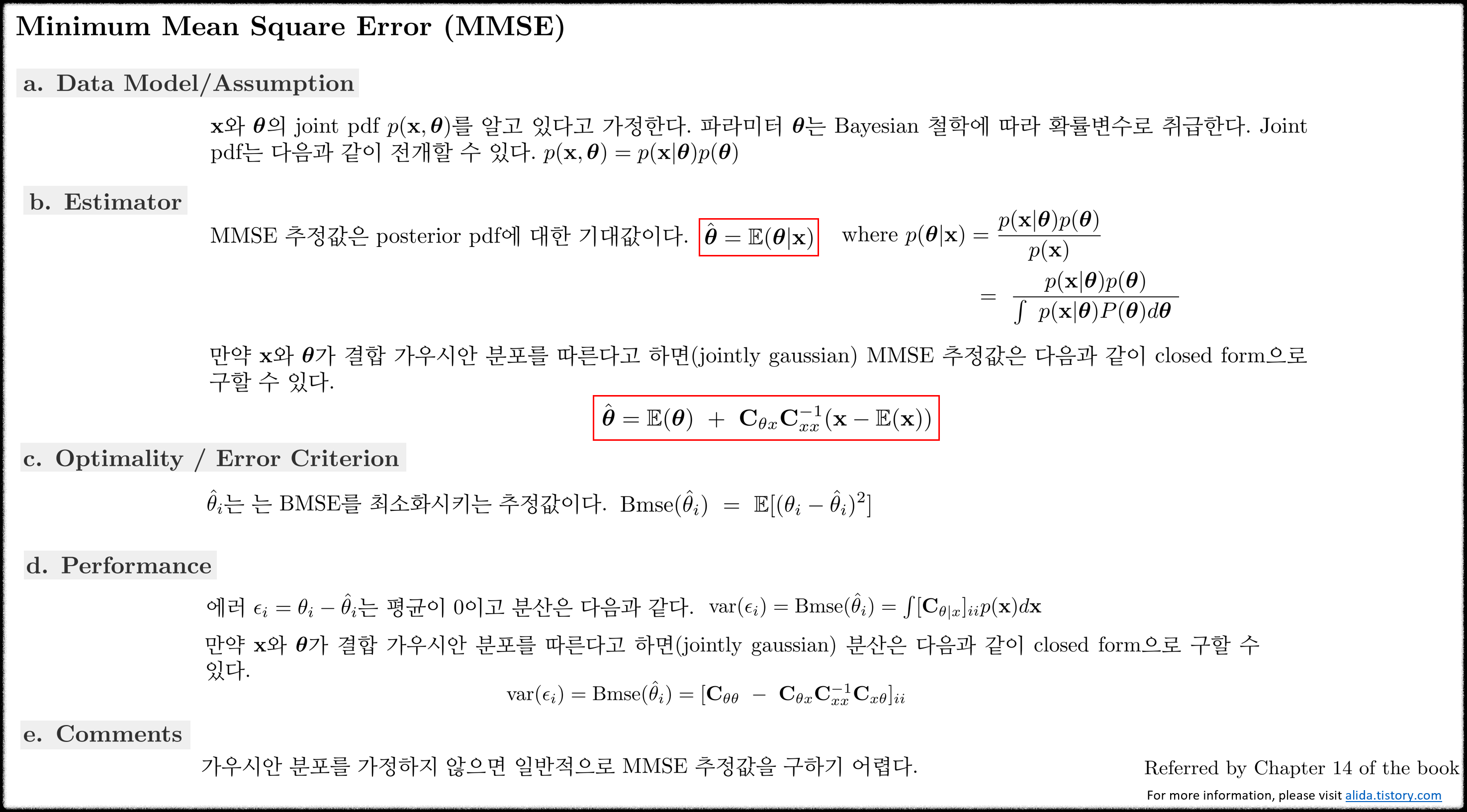
References

[1] Kay, Steven M. Fundamentals of statistical signal processing: estimation theory. Prentice-Hall, Inc., 1993.

[2] Simon, Dan. Optimal state estimation: Kalman, H infinity, and nonlinear approaches. John Wiley & Sons, 2006.

저작자표시

'Fundamental' 카테고리의 다른 글

확률 이론(Probability Theory) 개념 정리 Part 2 - Random Process, Gaussian Process (0)	2024.02.27
추정 이론(Estimation Theory) 개념 정리 Part 3 - Bayesian Philosophy (15)	2024.02.17
추정 이론(Estimation Theory) 개념 정리 Part 1 - MVUE, CRLB (1)	2024.02.10
[Math] Useful Mathematical Identities and Tricks 정리 (2)	2024.02.04
확률 이론(Probability Theory) 개념 정리 Part 1 - Probability, Random Variable, Distribution (1)	2023.11.13

추정 이론(Estimation Theory) 개념 정리 Part 2 - RBLS, BLUE, MLE, LSE, Exponential Familiy

5. General Minimum Variance Unbiased Estimation

5.1. Sufficient Statistics

5.1.1. Example 5.1 - Verification of a Sufficient Statistic

5.2. Finding Sufficient Statistics

5.2.1. Theorem 5.1 (Neyman-Fisher Factorization)

5.2.2. Example 5.2 - DC Level in WGN

5.2.3. Proof of the Neymann-Fisher Factorization

5.3. Using Sufficiency to Find the MVU Estimator

5.3.1. Example 5.5 - DC Level in WGN

5.3.2. Theorem 5.2 (Rao-Blackwell-Lehmann-Scheffe)

5.3.3. Example 5.6 - Completeness of a Sufficient Statistic

5.3.4. Example 5.7 - Incomplete Sufficient Statistic

5.4. Extension to a Vector Parameter

5.4.1. Example 5.10 and Example 5.11 - DC Level in WGN with Unknown Noise Power

6. Best Linear Unbiased Estimation

6.1. Definition of the BLUE

6.2. Finding the BLUE

6.2.1. Example 6.1 - DC Level in White Noise

6.3. Extension to a Vector Parameter

6.3.1. Theorem 6.1 (Gauss-Markov Theorem)

7. Maximum Likelihood Estimation

7.1. An Example

7.1.1. Example 7.1 - DC Level in White Gaussian Noise - Modified

7.2. Finding the MLE

7.2.1. Example 7.2 and 7.3 - DC Level in White Gaussian Noise - Modified (continued)

7.3. Properties of the MLE

7.3.1. Theorem 7.1 (Asymptotic Properties of the MLE)

8. Least Squares

8.1. The Least Squares Approach

8.1.1. Example 8.1 - DC Level Signal

8.2. Linear Least Squares

Scalar Case:

Vector Case:

Vector Weighted Case:

8.3. Geometrical Interpretations

8.3. Sequential Least Squares

Sequential LS (scalar parameter):

WLS $\rightarrow$ Sequential LS:

WLS $\rightarrow$ Sequential LS (vector parameter):

8.4. Constrained Least Squares

8.5. Nonlinear Least Squares

8.5.1. General approach for nonlinear LS

Newton-Raphson iteration:

Gauss-Newton iteration:

9. Exponential family

9.1. Exponential Family 1 - Bernoulli distribution

9.2. Exponential Family 2 - Gaussian distribution

9.3. Maximum Likelihood Estimator and Sufficient Statistics

Wrap up

References

'Fundamental' 카테고리의 다른 글

'Fundamental' Related Articles

티스토리툴바