 A L I D A
확률 이론의 기본적인 내용에 대해 알고 싶으면 확률 이론(Probability Theory) 개념 정리 Part 1 포스팅을 참조하면 된다.
NOMENCLATURE of Probability Theory
- 확률(probability)는 $Pr(\cdot)$으로 표기한다.
- 사건(event)은 대문자로 표기힌다. e.g., $A,B$
- 이산 확률질량함수(pmf)와 연속 확률밀도함수(pdf)는 각각 $P(\cdot)$와 $p(\cdot)$으로 표기한다.
- 확률변수(random variable)는 소문자로 표기한다. e.g., $x,y$
- 확률의 파라미터는 사건(event)이고 pdf, pmf의 파라미터는 확률변수가 된다. e.g., $Pr(A), P(x), p(x)$
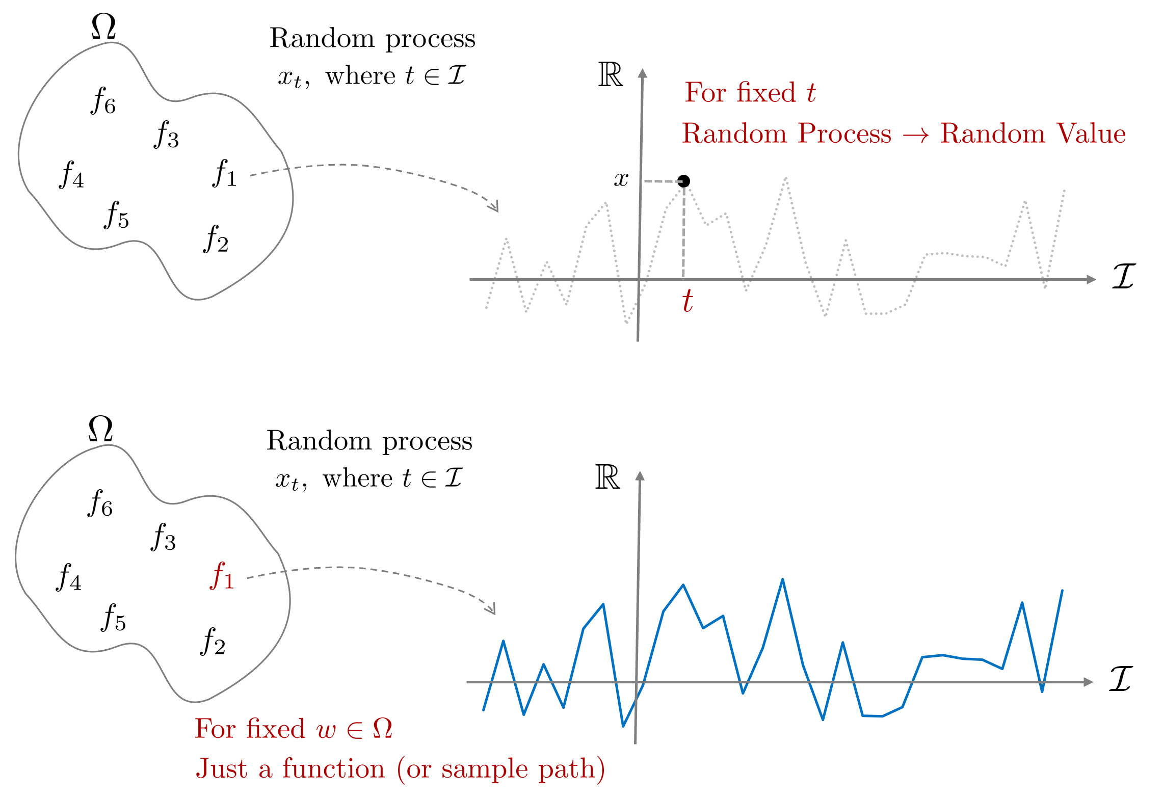
Random Process
랜덤 프로세스(random process)는 확률변수(random variable)을 무한차원으로 확장한 버전으로 생각하면 된다. 지금까지 배운 확률변수 $x$는 표본공간 $\Omega$에서 하나의 표본을 하나의 실수로 변환해주는 연산자의 역할을 수행하였다. 벡터 확률변수 $\mathbf{x} \in \mathbb{R}^{n}$을 생각해보면 표본공간 $\Omega$에서 $n$개의 표본을 $n$개의 실수 벡터로 변환하는 연산자의 역할을 수행하였다. 만약 $n$을 무한으로 확장하면 어떻게 될까?

$n \rightarrow \infty$가 된다면 벡터 확률변수 $\mathbf{x}$는 표본공간 $\Omega$에서 $\infty$개의 표본을 $\infty$개의 실수 벡터로 변환하는 연산자가 될 것이다. 이는 표본공간 $\Omega$에서 하나의 함수를 변환하는 연산자로 볼 수 있을 것이다. 함수해석학적으로 봤을 때 함수 $y=f(x)$는 $x$를 넣으면 $y$가 나오는 무한차원의 벡터로 해석할 수 있다. 예를 들어, 입출력이 실수라면 $x$도 무한개 $y$도 무한개인 벡터가 된다.
\begin{equation}
\begin{aligned}
f \Bigg( \begin{bmatrix}
x_1 \\ x_2 \\ \vdots \\ x_\infty
\end{bmatrix} \Bigg) = \begin{bmatrix}
y_1 \\ y_2 \\ \vdots \\ y_\infty
\end{bmatrix}
\end{aligned}
\end{equation}

따라서 랜덤프로세스는 표본공간 $\Omega$에서 랜덤한 함수 하나를 추출하는 과정으로 해석될 수 있으며 여기에서 인덱스 집합 $\mathcal{I}$를 사용하여 추가적인 차원 (일반적으로 시간 $t$)을 더해줌으로써 $\Omega \times \mathcal{I}$ 공간에서 원소를 추출하게 된다.

Definition of random process
랜덤 프로세스는 다음과 같은 기호로 표기한다.
\begin{equation}
\begin{aligned}
x_t(w), \quad \text{where, } t \in \mathcal{I}
\end{aligned}
\end{equation}
- $\mathcal{I}$ : 인덱스 집합(Index set). 일반적으로 시간(t)으로 간주한다.
이는 $t$의 존재만 제외하고는 앞서 정의한 확률변수 $x$와 동일하다. $t$는 일반적으로 시간으로 간주한다.
- 랜덤 프로세스는 표본공간 $\Omega$에서 하나의 원소를 뽑았을 때 함수들의 공간으로 매핑되는 연산으로 해석할 수 있다.\begin{equation}
\begin{aligned}
x_t : \Omega \rightarrow \text{ the set of all sequences or functions}
\end{aligned}
\end{equation} - 함수에 인덱스를 표기하기 위해(=축을 표기하기 위해) 인덱스 집합(index set)을 사용한다. \begin{equation}
\begin{aligned}
x_t : \mathcal{I} \rightarrow \text{ set of all random variables defined on } \Omega
\end{aligned}
\end{equation}
위 둘을 합하여 최종적으로 다음과 같이 표기한다. \begin{equation} \label{eq:rp1}
\boxed{ \begin{aligned}
x_t : \Omega \times \mathcal{I} \rightarrow \mathbb{R}
\end{aligned} }
\end{equation}
위 식에서 보다시피 랜덤프로세스는 표본공간과 인덱스 집합(일반적으로 시간 $t$)의 두 집합을 곱한 후(cartesian product) 하나의 실수 값을 반환하는 연산자로 볼 수 있다.
표본집합 $\Omega$에만 무작위성(randomness)가 존재하고 인덱스 집합 $\mathcal{I}$은 존재하지 않기 때문에 인덱스 집합 $t \in \mathcal{I}$을 고정시킨다면 랜덤프로세스 $x_t(w)$는 확률변수가 된다. 반대로 표본공간 내 원소 $w \in \Omega$를 실현(realization)한다면 확률변수 $x(w)$는 하나의 실수값이 나오지만 랜덤프로세스 $x_t(w)$는 하나의 함수(function 또는 sample path)가 나오게 된다.
\begin{equation}
\begin{aligned}
&\text{For fixed } {\color{Mahogany}t} \in \mathcal{I} \rightarrow x_{{\color{Mahogany}t}}(w) \text{ is a random variable} \\
&\text{For fixed } {\color{Mahogany}w} \in \Omega \rightarrow x_t({\color{Mahogany}w}) \text{ is a deterministic function of t} \end{aligned}
\end{equation}
Kolmogorov existence theorem
무한 차원에 대한 확률을 수학적으로 표현하기에 앞서 우선 $k$개의 확률변수에 대한 확률을 정의해보자.
\begin{equation}
\begin{aligned}
Pr((x_{t_1}, \cdots, x_{t_k}) \in B) \text{ for any } B, k, \text{ and } t_1, \cdots, t_k
\end{aligned}
\end{equation}
위 식은 사건 $B$내에 존재하는 $k$개의 확률변수의 확률을 정의할 수 있음을 의미한다. 위 식에서 $k=1$인 경우 이는 스칼라 확률변수 $x$의 확률을 정의하는 것과 동일하며, $k \rightarrow \infty$인 경우 무한한 확률변수에 대한 확률을 정의하는 것과 동일하다. 따라서 무한 차원에 대한 확률변수를 정의하는 것이 아닌 가변적으로 변할 수 있는 $k$개의 확률변수에 대한 확률을 정의하는 것이 곧 랜덤프로세스에서 확률을 정의하는 것이 되며 이를 Kolmogorov existence theorem이라고 한다.
Types of random process
확률변수 $x$는 다루고자 하는 표본공간이 이산값(discrete-value)을 가지는가 연속값(continuous-value)을 가지는가에 따라 두 가지 타입으로 분류할 수 있었다. 하지만 랜덤프로세스는 인덱스 집합 $\mathcal{I}$의 타입도 고려해야 하기 때문에 다음과 같은 타입이 추가적으로 고려되어야 한다.
- Discrete-time (for $\mathcal{I}$)
- Continuous-time (for $\mathcal{I}$)
- Discrete-value
- Continuous-value
이를 조합하여 총 네 개의 타입이 존재한다.
- DTDV(discrete-time, discrete-value)
- DTCV(discrete-time, continuous-value)
- CTDV(continuous-time, discrete-value)
- CTCV(continuous-time, continuous-value)
이 때, 인덱스 집합은 반드시 시간(t)일 필요는 없음에 유의한다. 여러 차원을 가진 인덱스 집합이 입력으로 사용될 수 있다. 하지만 앞서 정의한 랜덤프로세스 정의 (\ref{eq:rp1})에 따라 출력은 1차원 실수값이 되어야 한다. 출력이 여러 차원인 랜덤 프로세스는 해당 문서에서는 다루지 않는다.
Wiener process (a.k.a Brownian motion)
액체나 기체 속에 미세입자를 넣었을 때 보이는 불규칙한 모션을 브라운 모션이라고 하는데 이는 대표적인 랜덤프로세스의 예시이다. Kolmogorov existence theorem에 따라 $t$초를 관측하면 $t$초의 인덱스 집합에 대한 sample path를 얻는 랜덤프로세스로 해석할 수 있다. $t$는 유한한 값으로 반드시 무한대일 필요가 없다.
Momentum
랜덤프로세스는 하나의 샘플 $w \in \Omega$을 샘플링하였을 때 하나의 함수 $x_t(w)$가 나오기 때문에 랜덤프로세스의 1,2차 모멘텀 또한 평균, 분산이 아닌 평균함수, 분산함수가 된다.
Mean function
랜덤프로세스의 1차 모멘텀은 평균함수가 된다. 확률변수에 기대값 $\mathbb{E}$를 취하면 하나의 실수값이 되듯이 랜덤프로세스에 기대값을 취하면 하나의 함수가 된다.
\begin{equation}
\boxed{ \begin{aligned}
m_x(t) \triangleq \mathbb{E}(x_t) = \begin{cases} \sum_x x p_{x_t}(x) \quad &\text{ discrete-valued} \\
\int x f_{x_t}(x) dx \quad & \text{ continuous-valued}
\end{cases}
\end{aligned} }
\end{equation}
Auto-correlation function (ACF)
서로 다른 두 시간 $t,s$에 대하여 ACF는 다음과 같이 정의한다. 이는 벡터 확률변수 $\mathbf{x} = [x_1, x_2]^{\intercal}$이 있을 때 $\mathbb{E}(x_1 x_2)$의 랜덤프로세스 버전으로 생각하면 된다.
접두어 auto는 라틴어로 self를 의미하는 autos에서 유래되었다. 따라서 auto-corrleation function은 시계열 내에서 자기 자신과의 상관관계 함수를 의미한다.
\begin{equation}
\boxed{ \begin{aligned}
\mathbf{R}_{xx}(t,s) \triangleq \mathbb{E}(x_t x_s) \end{aligned} }
\end{equation}
Auto-covariance function (ACVF)
확률변수에 공분산(coviance)가 있다면 랜덤프로세스에는 ACVF가 있다. 이는 벡터 확률변수 $\mathbf{x} = [x_1, x_2]^{\intercal}$이 있을 때 $\text{cov}(x_1, x_2) = \mathbb{E}[(x_1 - \mu_{x_1})(x_2 - \mu_{x_2})]$의 랜덤프로세스 버전으로 생각하면 된다.
\begin{equation}
\boxed{ \begin{aligned}
\mathbf{C}_{xx}(t,s) \triangleq \mathbb{E}[(x_t - m_x(t))( x_s - m_x(s)]
\end{aligned} }
\end{equation}
Cross-covariance function (CCVF)
서로 다른 두 랜덤프로세스 $x_t, y_t$에 대하여 CCVF는 다음과 같이 정의된다. 이는 두 확률변수 $x, y$이 있을 때 $\text{cov}(x, y) = \mathbb{E}[(x - \mu_{x})(y - \mu_{y})]$의 랜덤프로세스 버전으로 생각하면 된다.
\begin{equation}
\boxed{ \begin{aligned}
\mathbf{R}_{xy}(t,s) \triangleq \mathbb{E}[(x_t - m_x(t))( y_s - m_y(s)]
\end{aligned} }
\end{equation}
Momentum on gaussian process
확률변수에서 가우시안 분포는 1,2차 모멘트인 평균, 분산을 사용하여 모든 확률분포를 표현할 수 있다. 이를 확장하여 만약 랜덤프로세스가 가우시안 분포를 따르고 평균이 $0$이라면 앞서 설명한 네 개의 모멘텀 중 ACF만을 사용하여 가우시안 프로세스를 설명할 수 있다. 왜냐하면 ACVF에서 $m_x(t), m_x(s)$가 전부 $0$이 되기 때문이다.
\begin{equation}
\boxed{ \begin{aligned}
\mathbf{C}_{xx}(t,s) & \triangleq \mathbb{E}[(x_t - 0)(x_s - 0)] \\
& = \mathbb{E}(x_t x_s) \\
& = \mathbf{R}_{xx}(t,s) \qquad \cdots \text{ for Gaussian process w\ } m_x(t)=0
\end{aligned} }
\end{equation}
이는 가우시안 프로세스의 매우 중요한 특징 중 하나이다.
Stationary
랜덤프로세스는 표본공간에서 랜덤한 함수를 추출하는 과정이기 때문에 매우 다양한 모양의 함수(e.g., 값이 튀거나 무한대의 값을 갖거나)가 나올 수 있다. 랜덤프로세스에서 정상성(stationary)이란 수많은 종류의 함수들 중 통계적 성질이 시간 구간 $[t, t + \tau]$에서 변하지 않는 성질을 말한다. 즉, $[t, t+\tau]$ 구간에서 동일한 확률분포를 갖는 성질을 정상성이라고 하며 랜덤프로세스가 정상성을 갖는 경우 이를 특별히 정상프로세스(stationary process)라고 한다.
Strict-sense stationary (SSS)
협의의 정상성(strict-sense stationary, SSS)이란 다음과 같이 성질을 만족하는 랜덤프로세스를 말한다.
\begin{equation}
\begin{aligned}
Pr((x_{t_1}, x_{t_2}, \cdots, x_{t_k}) \in B) = Pr((x_{t_1 + \tau}, x_{t_2+\tau}, \cdots, x_{t_k+\tau})\in B)
\end{aligned}
\end{equation}
위 식에서 보다시피 SSS는 시간 $t$가 임의의 간격 $\tau$에 대하여 이동하여도 확률은 동일한 경우(=shift invariant)를 말한다. SSS에서 모든 $n$차 모멘트들은 정상성을 띄며 다음과 같다.
\begin{equation}
\begin{aligned}
& m_x(t+\tau) = m_x(t) \\
& \mathbf{R}_{xx}(t+\tau, s+\tau) = \mathbf{R}_{xx}(t,s) \\
& \mathbf{C}_{xx}(t+\tau, s+\tau) = \mathbf{C}_{xx}(t,s)
\end{aligned}
\end{equation}
Wide-sense stationary (WSS)
광의의 정상성(wide-sense stationary, WSS)란 SSS처럼 모든 $n$차 모멘트들이 정상성을 만족하는 것이 아닌 1차(평균), 2차(분산) 모멘트들만 정상성을 만족하는 경우를 말한다.
\begin{equation}
\begin{aligned}
& m_x(t+\tau) = m_x(t) \\
& \mathbf{R}_{xx}(t+\tau, s+\tau) = \mathbf{R}_{xx}(t,s) \\
\end{aligned}
\end{equation}
이 때, 'WSS'이면 '2차 모멘트가 정상성'을 띄지만 반대로 '2차 모멘트가 정상성'을 띄면 'WSS"이다라는 역은 성립하지 않음에 유의한다. SSS는 지나치게 제약적이고 조건이 엄격하기 때문에 일반적으로 WSS를 많이 사용한다.
SSS, WSS 모두 임의의 시간 $t$에 대하여 평균함수 $m_x(t)=m_x(t+\tau)$를 만족하기 때문에 이는 곧 평균함수가 상수인 것을 의미한다.
\begin{equation}
\boxed{ \begin{aligned}
& \mathbb{E}(x_t) = m_x(t) = m_x(t+\tau) = m_x = \text{ constant}.
\end{aligned} }
\end{equation}
그리고 ACF는 다음과 같이 두 시간 $t, s$ 차이에 의한 함수가 된다.
\begin{equation}
\boxed{ \begin{aligned}
\mathbf{R}_{xx}(t,s) & = \mathbf{R}_{xx}(t-s, 0) \qquad \cdots \text{ if } \tau = t-s \\
& = \mathbf{R}_{xx}(0, t-s) \\
& = \mathbf{R}_{xx}(\tau)
\end{aligned} }
\end{equation}
따라서 랜덤프로세스가 정상성을 띄면 모멘트들은 더 이상 절대 시간 $t$에 의존하지 않고 상대적인 시간 차이 $\tau$에만 의존하게 된다. 또한, 위 식은 입력 시간 $t,s$ 값이 얼마나 서로 상관관계를 가지고 있느냐는 물리적 의미를 지닌다. 만약 $\tau=t-s$에 대하여 $\tau$가 작을 때 $ \mathbf{R}_{xx}(\tau)$ 값이 크다면 짧은 시간동안 함수의 모양이 급격히 변하는 것을 의미하고 반대로 $ \mathbf{R}_{xx}$ 값이 작다면 짧은 시간동안 함수의 모양이 부드럽게 변하는 것을 의미한다.
가우시안 분포의 경우 1,2차 모멘트만으로 모든 확률분포를 설명할 수 있는 좋은 성질을 가지고 있기 때문에 일반적으로 가우시안 프로세스는 WSS라고 가정한다. 그리고 앞서 말했듯이 평균함수가 $0$이라면 가우시안 프로세스는 공분산 $ \mathbf{C}_{xx}$가 ACF $ \mathbf{R}_{xx}$가 되어 ACF만을 사용하여 전부 표현할 수 있기 때문에 이는 매우 유용한 특징이 된다.
\begin{equation}
\begin{aligned}
\mathbf{C}_{xx}(\tau) = \mathbf{R}_{xx}(\tau) \qquad \cdots \text{ for Gaussian process w/ } m_x(t)=0
\end{aligned}
\end{equation}
Gaussian Process
가우시안 프로세스(gaussian process, GP)는 프로세스 집합 내에 존재하는 임의의 확률변수들의 조합이 모두 결합 가우시안 분포(joint gaussian distribution)를 따르는 랜덤프로세스를 말한다. 결합확률분포는 가우시안이기 때문에 1,2차 모멘트를 사용하여 완벽하게 표현이 가능하다.
- 평균함수: $m_x(t) = \mathbb{E}(x_t)$
- 공분산함수: $k(t,s) = \mathbf{C}_{xx}(t, s)$
위 식을 정리하여 랜덤프로세스 $x_t$가 GP를 따른다고 하면 일반적으로 다음과 같이 표기한다.
\begin{equation}
\boxed{ \begin{aligned}
x_t \sim \mathcal{G}\mathcal{P}(m_x(t), k(t,s))
\end{aligned} }
\end{equation}
Joint gaussian distribution
두 벡터 확률변수 $\mathbf{x} \in \mathbb{R}^{n}$이고 $\mathbf{y} \in \mathbb{R}^{m}$가 주어졌을 때 결합확률분포(joint probability distribtuion)는 다음과 같이 나타낼 수 있다.
\begin{equation} \boxed{ \begin{aligned} p(\mathbf{x},\mathbf{y}) = \frac{1}{(2\pi)^{\frac{n+m}{2}}\text{det}^{\frac{1}{2}}(\mathbf{C})}\exp \Bigg( -\frac{1}{2}\bigg(\begin{bmatrix} \mathbf{x} - \mathbb{E}(\mathbf{x}) \\ \mathbf{y} - \mathbb{E}(\mathbf{y}) \end{bmatrix}\bigg)^{\intercal}\mathbf{C}^{-1}\bigg(\begin{bmatrix} \mathbf{x} - \mathbb{E}(\mathbf{x}) \\ \mathbf{y} - \mathbb{E}(\mathbf{y}) \end{bmatrix}\bigg) \Bigg) \end{aligned} } \end{equation} 평균 벡터은 $\begin{bmatrix} \mathbb{E}(\mathbf{x})^{\intercal} & \mathbb{E}(\mathbf{y})^{\intercal} \end{bmatrix}^{\intercal} \in \mathbb{R}^{n+ m}$이고 공분산 행렬은 다음과 같다. \begin{equation} \begin{aligned} \mathbf{C} = \begin{bmatrix} \mathbf{C}_{xx} & \mathbf{C}_{xy} \\ \mathbf{C}_{yx} & \mathbf{C}_{yy} \end{bmatrix} = \begin{bmatrix} n\times n & n\times m \\ m\times n & m\times m \end{bmatrix} \in \mathbb{R}^{(n+m)\times (n+m)} \end{aligned} \end{equation}
앞서 랜덤프로세스에서 시간을 고정하면 이는 확률변수가 된다고 배웠다. 또한 GP는 정의에 따라 $t=1,3,5$로 시간을 고정하면 각각의 확률변수 $x_1, x_3, x_5$가 모두 결합 가우시안 분포를 따라야 한다(jointly gaussian). 시간을 고정하여 $\mathbf{x}=[x_1, x_3, x_5]^{\intercal}$이 얻어지면 결합 가우시안 분포는 다음과 같다.
\begin{equation} \begin{aligned} p(x_1, x_2, x_3) = \frac{1}{\sqrt{(2\pi)^{n}\text{det}^{\frac{1}{2}}(\mathbf{C})}}\exp \Bigg( -\frac{1}{2}\bigg(\begin{bmatrix} x_1 - \mathbb{E}(x_1) \\ x_2 - \mathbb{E}(x_2) \\ x_3 - \mathbb{E}(x_3) \end{bmatrix}\bigg)^{T}\mathbf{C}^{-1}\bigg(\begin{bmatrix} x_1 - \mathbb{E}(x_1) \\ x_2 - \mathbb{E}(x_2) \\ x_3 - \mathbb{E}(x_3) \end{bmatrix}\bigg) \Bigg) \end{aligned} \end{equation}
Toy example of gaussian process
예를 들어 $x_t = tA$이고 $A \sim \mathcal{N}(0,1)$, $t \in \mathbb{R}$을 만족하는 GP가 주어졌다고 가정하자.
해당 문제가 GP인지 확인하는 방법은 다음과 같다. GP는 시간이 고정되었을 때 확률변수가 되어야 한다고 했다. 만약 $t$가 고정되면 $x_n = nA$인 확률변수가 된다. 반대로 확률변수가 고정되면 이는 시간에 대한 함수가 된다. $A$가 확률변수가 아닌 고정된 값 $A_0$라고 하면 $x_t = t A_0$가 되어 이는 시간에 대한 함수가 된다.
다음으로 평균함수를 확인해보자.
\begin{equation}
\begin{aligned}
m_x(t) = \mathbb{E}(x_t) = t \mathbb{E}(A) = 0
\end{aligned}
\end{equation}
보다시피 평균은 $0$이 된다. 다음은 공분산함수를 확인해보자.
\begin{equation}
\begin{aligned}
k(t,s) = \mathbb{E}(tA sA) = ts \mathbb{E}(A^2) = ts
\end{aligned}
\end{equation}
따라서 이는 다음과 같이 다시 쓸 수 있다.
\begin{equation}
\begin{aligned}
x_t \sim \mathcal{G}\mathcal{P}(0, ts)
\end{aligned}
\end{equation}
공분산함수를 자세히 보면 이는 $t,s$에 대한 차이의 함수가 아닌 $t$와 $s$의 곱으로 이루어져 있다. 따라서 이 문제는 GP이지만 WSS가 아닌 것을 알 수 있다.
Gaussian Process Regression
가우시안 프로세스 회귀(gaussian process regression, GPR)은 가우스인 프로세스(GP)와는 다른 개념이다. GP는 랜덤프로세스의 한 종류를 말하는 반면에 GPR은 GP에 비모수적인 베이지안 방법(non-parametric bayesian method)을 적용하여 회귀 분석에 사용하는 알고리즘을 말한다.
\begin{equation}
\begin{aligned}
\text{GPR } = \text{ GP } + \text{ Non-parametric Bayesian method}
\end{aligned}
\end{equation}
GPR에서 자주 사용되는 기호(notation)의 의미는 다음과 같다.
- $\mathcal{I}$: 인덱스 집합 (e.g., 시간 $t \in \mathbf{R}$ 또는 공간 $\mathbf{R}^{n}$)
- $x_t$ : $t\in \mathcal{I}$일 때 여러 인덱스 값에 대응하는 확률변수들의 집합(collection)
- 가변적인 인덱스 집합 $\{t_1, t_2, \cdot, t_n\}$이 주어졌을 때 $\{ x_{t_1}, x_{t_2}, \cdots, x_{t_3} \}$가 평균이 $\mu \in \mathbb{R}^{n}$이고 공분산이 $K \in \mathbb{R}^{n \times n}$인 결합 가우시안 분포를 따른다면 $x_t$는 가우시안 프로세스라고 한다. 이 때, 평균과 공분산은 가변적인 인덱스 집합의 길이에 따라 달라진다.
GPR을 바라보는(=유도하는) 과정에 따라 weight-space view와 function-space view라는 두 개의 관점이 존재한다. Weight-space view는 수학적으로 길고 복잡한 유도과정이 전개되는 반면에 function-space view는 상대적으로 단순하게 최종 식이 유도된다. 다음 섹션부터는 weight-space view와 function space view를 설명하고 두 관점이 모두 동일한 결과를 유도함을 설명한다.
Weight-space view
Linear regression (MLE)
다음과 같은 간단한 선형 회귀 문제를 생각해보자.
\begin{equation}
\begin{aligned}
f(\mathbf{x}) = \mathbf{x}^{\intercal}\mathbf{w}
\end{aligned}
\end{equation}
위 식에서 우리는 관측 데이터 $\mathbf{x}$에 대한 파라미터(또는 가중치, weight) $\mathbf{w}$를 찾고자 한다. 만약 관측된 데이터에 노이즈가 섞여 있다면 식은 다음과 같이 쓸 수 있다.
\begin{equation}
\begin{aligned}
y(\mathbf{x}) = f(\mathbf{x}) + \epsilon \qquad \text{ where, } \epsilon \sim \mathcal{N}(0, \sigma^2_n)
\end{aligned}
\end{equation}
우리는 $n$개의 입력-출력 데이터 쌍 $\mathcal{D} = \{(x_i, y_i)\}_{i=1}^{n}$을 가지고 있다고 가정하자. $\mathbf{X} = \{ \mathbf{x}_1, \mathbf{x}_2, \cdots, \mathbf{x}_n \}$이라고 했을 때 likelihood는 다음과 같이 나타낼 수 있다.\begin{equation}
\begin{aligned}
p(\mathbf{y} | \mathbf{X}, \mathbf{w}) & = \Pi_{i=1}^{n} p(y_i | \mathbf{x}_i, \mathbf{w}) \\
& = \Pi_{i=1}^{n} \frac{1}{\sqrt{2\pi\sigma^2_n}} \exp\bigg( - \frac{(y_i - \mathbf{x}_i^{\intercal}\mathbf{w} )^2}{2\sigma^2_n} \bigg) \\
& = \frac{1}{(2\pi\sigma^2_n)^{n/2} } \exp \bigg( - \frac{1}{2\sigma^2_n} {\color{Mahogany} \| \mathbf{y} - \mathbf{X}^{\intercal} \mathbf{w} \|^2 } \bigg) \\
& \sim \mathcal{N}(\mathbf{X}^{\intercal}\mathbf{w}, \sigma^2_n \mathbf{I})
\end{aligned}
\end{equation}
Maximum likelihood estimation(MLE)를 사용하여 $\mathbf{w}$ 값을 추정해보면 위 식은 결국 다음 항을 최소화하는 최적화 문제가 된다.
\begin{equation}
\begin{aligned}
\mathbf{w}^{*} = \arg\min_{\mathbf{w}} {\color{Mahogany} \| \mathbf{y} - \mathbf{X}^{\intercal} \mathbf{w} \|^2 }
\end{aligned}
\end{equation}
위 식은 최소제곱법의 정규방정식을 사용하여 다음과 같이 해를 구할 수 있다.
\begin{equation}
\boxed{ \begin{aligned}
\mathbf{w}^{*} = (\mathbf{XX}^{\intercal})^{-1} \mathbf{X}^{\intercal} \mathbf{y} \qquad \cdots \text{ for linear regrssion}
\end{aligned} }
\end{equation}
Bayesian linear regression (MAP)
앞서 설명한 선형 회귀 문제는 고전적인 빈도론자(frequentist)의 추정 방법인 MLE을 사용하여 해를 도출하였다. 이와 달리 베이지만 추정 방법은 무엇이 다를까? 베이지안 추정 방법은 찾고자 하는 파라미터 $\mathbf{w}$가 결정된 값(deterministic value)가 아닌 하나의 확률변수(random variable)로 보고 $\mathbf{w}$의 사전 분포(prior pdf)를 고려할 수 있다는 점이 추가된다. $\mathbf{w}$를 평균이 $0$인 가우시안 분포를 따른다고 가정해보자.
\begin{equation}
\begin{aligned}
\mathbf{w} \sim \mathcal{N}(0, \Sigma_{w})
\end{aligned}
\end{equation}
이 때, 베이지안 방법론은 likelihood가 아닌 posterior pdf를 찾는 것이 목표가 된다.
\begin{equation}
\begin{aligned}
p(\mathbf{w} | \mathbf{y}, \mathbf{X}) & = \frac{p(\mathbf{y}|\mathbf{X},\mathbf{w}) p(\mathbf{w})}{p(\mathbf{y} | \mathbf{X})} \\
& = \eta \cdot p(\mathbf{y}|\mathbf{X},\mathbf{w}) p(\mathbf{w})
\end{aligned}
\end{equation}
Posterior pdf를 최대화하는 $\mathbf{w}$를 찾기 위해서는 maximum a posterior(MAP) 추정을 사용해야 한다.
\begin{equation}
\begin{aligned}
p(\mathbf{w} | \mathbf{y}, \mathbf{X}) & = \eta \cdot p(\mathbf{y}|\mathbf{X},\mathbf{w}) p(\mathbf{w}) \\
& \propto \exp \bigg( \frac{1}{2\sigma^2_n} (\mathbf{y}-\mathbf{X}^{\intercal}\mathbf{w})^{\intercal}(\mathbf{y}-\mathbf{X}^{\intercal}\mathbf{w}) \bigg) \exp \bigg( -\frac{1}{2} \mathbf{w}^{\intercal} \Sigma^{-1}_{w} \mathbf{w} \bigg) \\
& \propto \exp\bigg( \frac{1}{2}(\mathbf{w}-\bar{\mathbf{w}})^{\intercal}\mathbf{A}^{-1}(\mathbf{w}-\bar{\mathbf{w}}) \bigg)
\end{aligned}
\end{equation}
- $\bar{\mathbf{w}} = \frac{1}{\sigma^2_n} \mathbf{A} ^{-1}\mathbf{X}\mathbf{y}$
- $\mathbf{A} = \bigg( \frac{1}{\sigma^2_n}\mathbf{XX}^{\intercal} + \Sigma^{-1}_{w} \bigg)$
따라서 posterior pdf는 $p(\mathbf{w} | \mathbf{y}, \mathbf{X}) \sim \mathcal{N}(\bar{\mathbf{w}}, \mathbf{A} )$인 가우시안 분포를 따른다. MAP은 posterior pdf를 최대가 되는 평균이기 때문에 다음과 같이 구할 수 있다.
\begin{equation}
\boxed{ \begin{aligned}
\hat{\mathbf{w}}_{\text{MAP}} = \bar{\mathbf{w}} = \frac{1}{\sigma^2_n} \bigg( \frac{1}{\sigma^2_n} \mathbf{XX}^{\intercal} + \Sigma^{-1}_{w} \bigg)^{-1} \mathbf{X}^{\intercal} \mathbf{y} \qquad \cdots \text{ for bayesian linear regrssion}
\end{aligned} }
\end{equation}
만약 위 식에서 $\Sigma_{w}^{-1} \rightarrow 0$이 되면 MAP는 MLE와 동일한 형태가 된다. 이는 사전 정보에 대한 불확실성이 매우 클 때($\Sigma_{w} \rightarrow \infty$) MAP은 곧 MLE가 됨을 의미한다.
가우시안이 아닌 일반적인 분포의 경우 posterior pdf를 위와 같이 해석적(analytical)으로 푸는 것이 매우 어렵거나 불가능할 수 있다. 보통 $\mathbf{w}$의 사전 정보(prior)를 정확히 아는 것은 매우 어렵기 때문에 공액사전정보(conjugate prior)를 사용하여 수식을 유도한다. 이 때, 가우시안의 conjugate prior는 역시 가우시안이기 때문에 posterior를 깔끔하게 유도할 수 있다. 따라서 가우시안 분포를 일반적으로 많이 가정하여 사용한다.
Gaussian process regression
앞서 정의한 선형 회귀 문제를 다시 생각해보자.
\begin{equation} \label{eq:gpr3}
\begin{aligned}
f(\mathbf{x}) = \mathbf{x}^{\intercal} \mathbf{w}
\end{aligned}
\end{equation}
- $y(\mathbf{x}) = f(\mathbf{x}) + \epsilon \quad \text{ where } \epsilon \sim \mathcal{N}(0, \sigma^2_{n})$
- $\mathbf{w} \sim \mathcal{N}(0, \Sigma_{w})$
만약 $\mathbf{x}, \mathbf{w}$가 모두 가우시안 분포를 따른다고 하고 평균함수와 공분산함수를 구해보면 다음과 같다.
\begin{equation}
\begin{aligned}
& \mathbb{E}(f(\mathbf{x})) = \mathbf{x}^{\intercal}\mathbb{E}(\mathbf{w}) = 0 \\
& \mathbb{E}(f(\mathbf{x})f(\mathbf{x}')) = \mathbf{x}^{\intercal} \mathbb{E}(\mathbf{ww}^{\intercal})\mathbf{x}' = \mathbf{x}^{\intercal} \Sigma_w \mathbf{x}' = k(\mathbf{x}, \mathbf{x}')
\end{aligned}
\end{equation}
위 식에서 보다시피 선형 회귀 문제는 모든 변수들 $[f(\mathbf{x}_1), \cdots, f(\mathbf{x}_n)]$이 결합 가우시안 분포를 따르므로 평균함수가 $0$이고 공분산이 $k(\mathbf{x}, \mathbf{x}')$ 가우시안 프로세스 문제로 해석할 수 있다.
Predictive distribution
우리는 앞서 베이지안 추정을 사용하여 MAP 추정값을 얻었다. 하지만 우리가 관심있는 부분은 새로운 입력 $\mathbf{x}_{*}$가 들어 왔을 때 출력값 $f_{*}=\mathbf{x}_*^{\intercal} \mathbf{w}$가 어떻게 되는가이다. 출력값을 예측하기 위해 다음과 같은 예측분포(predictive distribution)를 정의할 수 있다.
\begin{equation}
\begin{aligned}
p(f_* | \mathbf{x}_*, \mathbf{X}, \mathbf{y}) & = \int p(f_* | \mathbf{x}_*, \mathbf{w}) p(\mathbf{w} | \mathbf{X}, \mathbf{y}) d \mathbf{w} \\
& \sim \mathcal{N}\bigg(\frac{1}{\sigma^2_n}\mathbf{x}_*^{\intercal} \mathbf{A}^{-1}\mathbf{X}\mathbf{y}, \mathbf{x}_*^{\intercal}\mathbf{A}^{-1}\mathbf{x}_* \bigg)
\end{aligned}
\end{equation}
출력값이 $f_{*}=\mathbf{x}_*^{\intercal} \mathbf{w}$이기 때문에 기존 $\mathbf{w}$가 평균 $\mathcal{N}(\mathbf{a},\mathbf{B})$를 따른다면 $f_*$는 $\mathcal{N}(\mathbf{x}_*\mathbf{a}, \mathbf{x}_*^{\intercal}\mathbf{B}\mathbf{x}_*)$를 따르는 것을 알 수 있다.
Kernel trick
예측분포의 평균과 분산을 구하기 위해 커널 트릭(kernel trick)을 사용해보자. 커널 트릭은 입력 데이터를 고차원 특성 공간으로 매핑하는 함수를 사용한다. 이 고차원 공간에서는 원래의 비선형 문제가 선형적으로 더 잘 분리될 수 있다. 커널 함수는 이러한 고차원 공간에서의 내적을 직접 계산하는 것과 동일한 결과를 제공하지만, 실제로 데이터를 고차원으로 변환하지 않기 때문에 계산 비용을 크게 절감할 수 있다.
커널 함수는 $\phi : \mathbb{R}^{D} \rightarrow \mathbb{R}^{N}$와 같이 기존의 관측 데이터를 고차원으로 매핑시켜주는 함수이다($N \gg D$). 커널 함수를 사용하여 기존 회귀 문제를 다음과 같이 바꿀 수 있다.
\begin{equation}
\begin{aligned}
f(\mathbf{x}) = \phi(\mathbf{x})^{\intercal} \mathbf{w}
\end{aligned}
\end{equation}
위 문제의 평균함수와 공분산함수는 다음과 같다.
\begin{equation}
\begin{aligned}
& \mathbb{E}(f(\mathbf{x})) = \phi(\mathbf{x})^{\intercal}\mathbb{E}(\mathbf{w}) = 0 \\
& \mathbb{E}(f(\mathbf{x})f(\mathbf{x}')) = \phi(\mathbf{x})^{\intercal} \mathbb{E}(\mathbf{ww}^{\intercal})\phi(\mathbf{x}') = \phi(\mathbf{x})^{\intercal} \Sigma_w \phi(\mathbf{x}') = k(\mathbf{x}, \mathbf{x}')
\end{aligned}
\end{equation}
위 식에서 보다시피 커널 함수를 적용해도 모든 변수들 $[f(\mathbf{x}_1), \cdots, f(\mathbf{x}_n)]$ 이 결합 가우시안 분포를 따르므로 평균함수가 $0$이고 공분산이 $k(\mathbf{x}, \mathbf{x}')$ 가우시안 프로세스 문제로 해석할 수 있다.
앞서 예측분포의 평균과 분산은 다음과 같았다.
\begin{equation}
\begin{aligned}
f_* | \mathbf{x}_*, \mathbf{X}, \mathbf{y} \sim \mathcal{N} \bigg(\frac{1}{\sigma^2_n}\mathbf{x}_*^{\intercal} \mathbf{A}^{-1}\mathbf{X}\mathbf{y}, \mathbf{x}_*^{\intercal} \mathbf{A}^{-1}\mathbf{x}_* \bigg)
\end{aligned}
\end{equation}
여기에 커널 함수를 적용하면 다음과 같이 변경된다.
\begin{equation} \label{eq:gpr1}
\begin{aligned}
f_* | \mathbf{x}_*, \mathbf{X}, \mathbf{y} \sim \mathcal{N}\bigg( \frac{1}{\sigma^2_n}\phi(\mathbf{x}_*)^{\intercal} \mathbf{A}^{-1}\Phi \mathbf{y}, \phi(\mathbf{x}_*)^{\intercal} \mathbf{A}^{-1} \phi(\mathbf{x}_*) \bigg)
\end{aligned}
\end{equation}
- $\Phi = \Phi(\mathbf{X}) = [ \phi(\mathbf{x}_1), \ \cdots, \ \phi(\mathbf{x}_n) ]^{\intercal} \in \mathbb{R}^{N \times n}$
- $\mathbf{A} = \bigg( \frac{1}{\sigma^2_n}\Phi \Phi^{\intercal} + \Sigma^{-1}_{w} \bigg) \in \mathbb{R}^{N \times N}$
커널 함수에 의해 차원이 $N$차원이 되었고 $N \gg D$이기 때문에 기존 $\mathbf{A}^{-1}$은 $D \times D$의 역행렬을 구하는 문제에서 더 큰 차원의 $N \times N$의 역행렬을 구하는 문제가 되었다. 이는 연산량의 증가로 이어진다.
이 문제를 해결하기 위해 변환 트릭을 사용한다. 우선 $\mathbf{K}=\Phi^{\intercal} \Sigma_w \Phi \in \mathbb{R}^{n\times n}$라고 하고 새로운 입력 $\mathbf{x}_*$에 대한 $\phi_* = \phi( \mathbf{x}_*)$라고 하면 $\mathbf{A} \Sigma_w \Phi$는 다음과 같이 전개할 수 있다.
\begin{equation}
\begin{aligned}
{\color{Cyan} \mathbf{A} \Sigma_w \Phi } & = (\sigma_n^{-2} \Phi\Phi^{\intercal} + \Sigma_w^{-1}) \Sigma_{w} \Phi \\
& = \sigma_n^{-2} \Phi {\color{Mahogany} \Phi^{\intercal} \Sigma_w \Phi } + \Phi \\
& = \sigma_n^{-2} \Phi ({\color{Mahogany} \Phi^{\intercal} \Sigma_w \Phi } + \sigma^2_n \mathbf{I}) \\
& = \sigma_n^{-2} \Phi ({\color{Mahogany} \mathbf{K} } + \sigma^2_n \mathbf{I})
\end{aligned}
\end{equation}
위 마지막 식 앞에 $\mathbf{A}^{-1}$을 곱하고 뒤에 $( \mathbf{K} + \sigma^2_n \mathbf{I})^{-1}$를 곱하면 식은 다음과 같이 전개된다.
\begin{equation}
\begin{aligned}
\sigma_n^{-2} \mathbf{A}^{-1} \Phi ( \mathbf{K} + \sigma^2_n \mathbf{I})( \mathbf{K} + \sigma^2_n \mathbf{I})^{-1} & = \mathbf{A}^{-1}{\color{Cyan} \mathbf{A} \Sigma_w \Phi } ( \mathbf{K} + \sigma^2_n \mathbf{I})^{-1} \\
\sigma_n^{-2} \mathbf{A}^{-1} \Phi & = \Sigma_w \Phi ( \mathbf{K} + \sigma^2_n \mathbf{I})^{-1}
\end{aligned}
\end{equation}
(\ref{eq:gpr1})에 위 식을 대입하면 평균은 다음과 같이 변경된다.
\begin{equation}
\begin{aligned}
\sigma_n^{-2} \phi_*^{\intercal} \mathbf{A}^{-1}\Phi \mathbf{y} = {\color{Blue} \phi_*^{\intercal} \Sigma_w \Phi ( \mathbf{K} + \sigma^2_n \mathbf{I})^{-1} \mathbf{y} }
\end{aligned}
\end{equation}
Matrix inversion lemma를 사용하면 분산은 다음과 같이 변경된다.
\begin{equation}
\begin{aligned}
\phi_*^{\intercal} \mathbf{A}^{-1}\phi_* = {\color{Red} \phi_*^{\intercal} \Sigma_w \phi_* - \phi_*^{\intercal} \Sigma_w \Phi ( \mathbf{K} + \sigma^2_n \mathbf{I})^{-1} \Phi^{\intercal} \Sigma_w \phi_* }
\end{aligned}
\end{equation}
둘을 합치면 (\ref{eq:gpr1})식은 다음과 같이 변경된다.
\begin{equation} \label{eq:gpr2}
\begin{aligned}
f_* | \mathbf{x}_*, \mathbf{X}, \mathbf{y} \sim \mathcal{N}\bigg( & {\color{Blue} \phi_*^{\intercal} \Sigma_w \Phi ( \mathbf{K} + \sigma^2_n \mathbf{I})^{-1} \mathbf{y} } , \\
& {\color{Red} \phi_*^{\intercal} \Sigma_w \phi_* - \phi_*^{\intercal} \Sigma_w \Phi ( \mathbf{K} + \sigma^2_n \mathbf{I})^{-1} \Phi^{\intercal} \Sigma_w \phi_* } \bigg)
\end{aligned}
\end{equation}
위 식은 $N \times N$ 역행렬을 구하는 대신 $\phi_*$의 내적과 $n \times n$ 크기의 역행렬을 구하는 문제로 변경되었다. 일반적으로 $n < N$이기 때문에 동일한 평균과 분산을 효율적(=computaionally efficient)으로 구할 수 있다. 최종적으로 (\ref{eq:gpr2})에 커널 트릭을 표기법을 사용하여 $\phi( \mathbf{x} )^{\intercal} \Sigma_w \phi( \mathbf{x}' ) = k(\mathbf{x}, \mathbf{x}')$로 나타내면 새로운 입력에 대한 GPR의 평균과 분산을 구할 수 있다.
\begin{equation} \label{eq:gpr4}
\boxed{ \begin{aligned}
f_* | \mathbf{x}_*, \mathbf{X}, \mathbf{y} \sim \mathcal{N}\bigg( & {\color{Blue} k(\mathbf{x}_*, \mathbf{X}) ( k(\mathbf{X}, \mathbf{X}) + \sigma^2_n \mathbf{I})^{-1} \mathbf{y} } , \\
& {\color{Red} k(\mathbf{x}_*, \mathbf{x}_*) - k(\mathbf{x}_*, \mathbf{X}) ( k(\mathbf{X}, \mathbf{X}) + \sigma^2_n \mathbf{I})^{-1} k(\mathbf{X}, \mathbf{x}_*) } \bigg)
\end{aligned} }
\end{equation}
- $\phi_*^{\intercal} \Sigma_w \Phi = k(\mathbf{x}_*, \mathbf{X})$
- $\mathbf{K} = \Phi^{\intercal} \Sigma_w \Phi = k(\mathbf{X}, \mathbf{X})$
- $\phi_*^{\intercal} \Sigma_w \phi_* = k(\mathbf{x}_*, \mathbf{x}_*)$
- $\Phi^{\intercal} \Sigma_w \phi_* = k(\mathbf{X}, \mathbf{x}_*)$
Function-space view
(\ref{eq:gpr3})의 GPR 문제를 다시 생각해보자.
\begin{equation}
\begin{aligned}
f(\mathbf{x}) = \mathbf{x}^{\intercal} \mathbf{w}
\end{aligned}
\end{equation}
- $\mathbf{w} \sim \mathcal{N}(0, \Sigma_{w})$
만약 $\mathbf{w}$가 가우시안 분포를 따른다고 하고 평균함수와 공분산함수를 구해보면 다음과 같다.
\begin{equation}
\begin{aligned}
& \mathbb{E}(f(\mathbf{x})) = \mathbf{x}^{\intercal}\mathbb{E}(\mathbf{w}) = 0 \\
& \mathbb{E}(f(\mathbf{x})f(\mathbf{x}')) = \mathbf{x}^{\intercal} \mathbb{E}(\mathbf{ww}^{\intercal})\mathbf{x}' = \mathbf{x}^{\intercal} \Sigma_w \mathbf{x}' = k(\mathbf{x}, \mathbf{x}')
\end{aligned}
\end{equation}
이는 평균함수가 $0$이고 공분산함수가 $k(\mathbf{x}, \mathbf{x}')$인 GP로 볼 수 있다. 따라서 $f(\mathbf{X}) = \begin{bmatrix} f(\mathbf{x}_1) & f(\mathbf{x}_2) & \cdots &f(\mathbf{x}_n) \end{bmatrix}^{\intercal} \in \mathbb{R}^{n}$의 모든 변수들은 다음과 같은 결합 가우시안 분포를 따른다.
\begin{equation}
\begin{aligned}
\begin{bmatrix} f(\mathbf{x}_1) \\ f(\mathbf{x}_2) \\ \vdots \\ f(\mathbf{x}_n) \end{bmatrix} \sim \mathcal{N} \Bigg( 0, \begin{bmatrix}
k(\mathbf{x}_1, \mathbf{x}_1) & \cdots & k(\mathbf{x}_1, \mathbf{x}_n) \\
\vdots & \ddots & \vdots \\
k(\mathbf{x}_n, \mathbf{x}_1) & \cdots & k(\mathbf{x}_n, \mathbf{x}_n) \\ \end{bmatrix} \Bigg)
\end{aligned}
\end{equation}
새로운 입력 $f(\mathbf{x}_*) \in \mathbb{R}$가 주어졌다고 해보자. 이 때, 기존 $f(\mathbf{X})$와 $ f(\mathbf{x}_*)$는 서로 결합 가우시안 분포를 따라야 하므로 이는 다음과 같이 확장하여 쓸 수 있다.
\begin{equation}
\begin{aligned}
\begin{bmatrix} f(\mathbf{x}_1) \\ f(\mathbf{x}_2) \\ \vdots \\ f(\mathbf{x}_n) \\ {\color{Mahogany} f(\mathbf{x}_*) } \end{bmatrix} \sim \mathcal{N} \Bigg( 0, \begin{bmatrix}
k(\mathbf{x}_1, \mathbf{x}_1) & \cdots & k(\mathbf{x}_1, \mathbf{x}_n) & {\color{Mahogany} k(\mathbf{x}_1, \mathbf{x}_*) } \\
\vdots & \ddots & \vdots & \vdots \\
k(\mathbf{x}_n, \mathbf{x}_1) & \cdots & k(\mathbf{x}_n, \mathbf{x}_n) & {\color{Mahogany} k(\mathbf{x}_n, \mathbf{x}_*) } \\
{\color{Mahogany} k(\mathbf{x}_*, \mathbf{x}_1) } & \cdots & {\color{Mahogany} k(\mathbf{x}_*, \mathbf{x}_n) } & {\color{Mahogany} k(\mathbf{x}_*, \mathbf{x}_*) } \\ \end{bmatrix} \Bigg)
\end{aligned}
\end{equation}
위 식을 간략하게 표현하면 다음과 같다.
\begin{equation} \label{eq:gpr5}
\boxed{ \begin{aligned}
\begin{bmatrix} \mathbf{f} \\ f_* \end{bmatrix} \sim \mathcal{N} \Bigg( 0, \begin{bmatrix}
k(\mathbf{X}, \mathbf{X}) & k(\mathbf{X}, \mathbf{x}_*) \\
k(\mathbf{x}_*, \mathbf{X}) & k(\mathbf{x}_*, \mathbf{x}_*) \\ \end{bmatrix} \Bigg)
\end{aligned} }
\end{equation}
우리는 $\mathbf{f}$가 주어졌을 때 새로운 값 $f_*$의 확률분포를 계산하고 싶으므로 이는 조건부 확률분포(conditional pdf) $p(f_* | \mathbf{x}_*, \mathbf{X}, \mathbf{f})$을 사용하여 문제를 풀 수 있다.
\begin{equation}
\begin{aligned}
f_* | \mathbf{x}_*, \mathbf{X}, \mathbf{f} \sim \mathcal{N} \bigg( & {\color{Blue} k(\mathbf{x}_*, \mathbf{X}) k(\mathbf{X},\mathbf{X})^{-1} \mathbf{f} } , \\
& {\color{Red} k(\mathbf{x}_*, \mathbf{x}_*) - k(\mathbf{x}_*,\mathbf{X}) k(\mathbf{X},\mathbf{X})^{-1} k(\mathbf{X}, \mathbf{x}_*) } \bigg)
\end{aligned}
\end{equation}
Conditional gaussian distribution
두 벡터 확률변수 $\mathbf{x}, \mathbf{y}$가 주어졌을 때 조건부 확률분포 $p(\mathbf{y}|\mathbf{x})$가 가우시안 분포를 따른다고 하면 \begin{equation} \begin{aligned} p(\mathbf{y}| \mathbf{x}) & = \frac{p(\mathbf{x},\mathbf{y})}{p(\mathbf{x})} = \frac{p(\mathbf{x} | \mathbf{y})p(\mathbf{y})}{p(\mathbf{x})} = \eta \cdot p(\mathbf{x}|\mathbf{y})p(\mathbf{y}) \\ & \sim \mathcal{N}(\mathbb{E}(\mathbf{y}|\mathbf{x}), \mathbf{C}_{y|x}) \end{aligned} \end{equation} 가 된다. 평균 $\mathbb{E}(\mathbf{y}|\mathbf{x})$과 분산 $\mathbf{C}_{y|x}$은 아래와 같다. \begin{equation} \boxed{ \begin{aligned} & \mathbb{E}(\mathbf{y}|\mathbf{x})= \mathbb{E}(\mathbf{y}) + \mathbf{C}_{yx}\mathbf{C}_{xx}^{-1}(\mathbf{x} - \mathbb{E}(\mathbf{x})) \\ & \mathbf{C}_{y|x} = \mathbf{C}_{yy} - \mathbf{C}_{yx}\mathbf{C}_{xx}^{-1}\mathbf{C}_{yx}^{\intercal} \end{aligned} } \end{equation}
위 식은 (\ref{eq:gpr4})와 상당히 유사한 것을 볼 수 있다. Function-space view에서는 관측 노이즈 $y(\mathbf{x}) = f(\mathbf{x}) + \epsilon \text{, where } \epsilon \sim \mathcal{N}(0, \sigma^2_n)$이 고려되지 않아서 이에 대한 항이 빠져 있는 점이 다르다. 만약 관측 노이즈를 고려하면 공분산함수는 다음과 같이 변경된다.
\begin{equation}
\begin{aligned}
\mathbf{C}_{xx}(f(\mathbf{x}_1), f(\mathbf{x}_2)) = k(\mathbf{x}_1, \mathbf{x}_2) + {\color{Cyan} \sigma^2_n }
\end{aligned}
\end{equation}
(\ref{eq:gpr5})에서 $k(\mathbf{X}, \mathbf{X})$의 자기 자신의 대각(diagonal) 성분만 $\sigma^2_n$이 살아남아서 $\sigma^2_n \mathbf{I}$가 된다.
\begin{equation}
\boxed{ \begin{aligned}
\begin{bmatrix} {\color{Cyan} \mathbf{y} } \\ f_* \end{bmatrix} \sim \mathcal{N} \Bigg( 0, \begin{bmatrix}
k(\mathbf{X}, \mathbf{X}) + {\color{Cyan} \sigma^2_n \mathbf{I} } & k(\mathbf{X}, \mathbf{x}_*) \\
k(\mathbf{x}_*, \mathbf{X}) & k(\mathbf{x}_*, \mathbf{x}_*) \\ \end{bmatrix} \Bigg)
\end{aligned} }
\end{equation}
최종적으로 function-space view에서도 (\ref{eq:gpr4})와 완전히 동일한 GPR 수식이 유도된다.
\begin{equation}
\boxed{ \begin{aligned}
f_* | \mathbf{x}_*, \mathbf{X}, {\color{Cyan} \mathbf{y} } \sim \mathcal{N}\bigg( & k(\mathbf{x}_*, \mathbf{X}) ( k(\mathbf{X}, \mathbf{X}) + {\color{Cyan} \sigma^2_n \mathbf{I} } )^{-1} {\color{Cyan} \mathbf{y} } , \\
& k(\mathbf{x}_*, \mathbf{x}_*) - k(\mathbf{x}_*, \mathbf{X}) ( k(\mathbf{X}, \mathbf{X}) + {\color{Cyan} \sigma^2_n \mathbf{I} } )^{-1} k(\mathbf{X}, \mathbf{x}_*) \bigg)
\end{aligned} }
\end{equation}
Pros and cons of GPR
GPR의 장점과 단점은 다음과 같이 요약할 수 있다.
Pros
- 원리적 접근: GPR은 데이터를 모델링하는 과정에서 수학적으로 엄밀하고 체계적인 방법을 제공한다.
- 확률적 예측: GPR은 단순한 예측값을 제공하는 것이 아니라, 예측의 불확실성을 포함한 확률적인 예측을 제공한다. 이는 의사결정 과정에서 유용한 정보를 제공한다.
- 예측 불확실성의 정량화: GPR은 예측에 대한 불확실성을 명확하게 산출할 수 있다. 이는 모델의 예측이 얼마나 정확할지에 대한 감을 준다.
Cons
- 연산량: 역행렬을 구하는 과정에서 $O(n^3)$의 시간복잡도가 발생하므로 연산량이 많다. 이를 해결하기 위해 다양한 연구가 이루어지고 있다.
References
[1] (Blog)평균과 기댓값
[2] (Blog) PRLM - 4. The Exponential Family
[3] (Blog) [수리통계학] 38. 지수족
[4] (Wiki) Law of total expectation
[6] (Lecture) Bayesian Deep Learning - 최성준
[7] Williams, Christopher KI, and Carl Edward Rasmussen. Gaussian processes for machine learning. Vol. 2. No. 3. Cambridge, MA: MIT press, 2006.


