Quaternion kinematics for the error-state Kalman filter 내용 정리 Part 2

3 Quaternion conventions. My choice

3.1 Quaternion flavors

쿼터니언은 다양한 표기법이 존재한다. 일반적으로 다음과 같이 4개의 선택지가 존재한다.

• 실수부와 허수부를 어디에 둘 것인가에 따라

$$\begin{array}{}\text{(1)}& \mathbf{q}=\left[\begin{array}{c}{q}_w\\ {\mathbf{q}}_v\end{array}\right]\text{vs.}\mathbf{q}=\left[\begin{array}{c}{\mathbf{q}}_v\\ q_w\end{array}\right]\end{array}$$

• 쿼터니언 대수학을 어떻게 정의하느냐에 따라

$$\begin{array}{}\text{(2)}& ij=-ji=k\text{vs.}ji=-ij=k\end{array}$$

이는 곧 오른손법칙, 왼손법칙과 관련이 있다.
$$\begin{array}{}\text{(3)}& \text{right-handed}\text{vs.}\text{left-handed}\end{array}$$

3차원 공간에서 임의의 축 $\mathbf{u}$가 주어졌을 때 이를 중심으로 ${\mathbf{q}}_{\text{right}}\{\mathbf{u}\theta \}$는 오른손법칙을 사용하여 벡터를 $\theta$만큼 회전시키고 ${\mathbf{q}}_{\text{left}}\{\mathbf{u}\theta \}$는 왼손법칙을 사용하여 벡터를 $\theta$만큼 회전시킨다.

• 회전 연산자로써 기능에 따라

$$\begin{array}{}\text{(4)}& \text{Passive}\text{vs.}\text{Active}\end{array}$$

프레임을 회전시키느냐, 벡터를 회전시키느냐 차이가 있다.

• 프레임을 회전시키는 Passive 케이스인 경우, 연산의 방향에 따라서

$$\begin{array}{}\text{(5)}& {\mathbf{x}}_{global}=\mathbf{q}\otimes {\mathbf{x}}_{local}\otimes {\mathbf{q}}^{\ast }\text{vs.}{\mathbf{x}}_{local}=\mathbf{q}\otimes {\mathbf{x}}_{global}\otimes {\mathbf{q}}^{\ast }\end{array}$$


위 경우의 수만 보더라도 총 12가지의 서로 다른 조합이 나온다. 최근 대표적으로 사용하는 규약(convention)은 Hamilton, STS, JPL, ISS, ESA, 로봇공학회 표기법 정도가 존재한다. 대부분의 규약들은 서로 미세한 차이를 가지고 있으나 자주 정확히 명시하지 않은 상태로 사용된다. 이러한 차이점은 실제 회전연산에 큰 차이를 가져오고 서로 호환이 불가능하기 때문에 어떤 쿼터니언 표기법을 사용하는지 명확한 설명이 필요하다.

가장 유명한 2개의 규약은 Hamilton 표기법과 JPL 표기법이다. JPL 표기법은 항공분야에서 주로 사용되는 반면, Hamilton 표기법은 로보틱스 분야에서 주로 사용된다. 필자는 본 페이퍼에 Hamilton 표기법을 사용하여 쿼터니언을 표기하였다. 이는 로보틱스에서 자주 사용하는 라이브러리인 Eigen, ROS, Ceres에서 채택한 쿼터니언 표기법이고 칼만필터를 이용한 IMU 상태 추정 자료에도 주로 Hamilton 표기법이 사용되기 때문이다. JPL은 Hamilton에 비해 상대적으로 로보틱스 분야에서 적게 사용된다.

3.1.1 Order of the quaternion components

Hamilton과 JPL의 가장 근본적인 차이는 아니지만 확연히 구분 가능한 차이는 쿼터니언 원소를 표기하는 순서이다. Hamilton은 스칼라 파트를 앞에 위치시키고 JPL은 뒤에 위치시킨다. 이러한 스칼라, 벡터의 표현 순서 차이는 명확히 구분 가능하나 해석의 어려움을 줄 정도로 큰 차이는 아니다. 예를 들어 Hamilton 표기법을 따르는 Eigen 라이브러리 또한 쿼터니언의 실수부를 맨 뒤에 위치시키는 경우가 존재한다. 일반적으로 쿼터니언 $\mathbf{q}$를 $(w,x,y,z)$라고 표기하면 $w$가 실수부이고 $x,y,z$가 허수부를 의미한다.

3.1.2 Specification of the quaternion algebra

Hamilton 표기법의 쿼터니언 대수 규칙은 다음과 같다. ($ij=k$)
$$\begin{array}{}\text{(6)}& i^2=j^2=k^2=ijk=-1,ij=-ji=k,jk=-kj=i,ki=-ik=j\end{array}$$

반면에, JPL 표기법의 쿼터니언 대수 규칙은 다음과 같다. ($ji=k$)
$$\begin{array}{}\text{(7)}& i^2=j^2=k^2=-ijk=-1,-ij=ji=k,-jk=kj=i,-ki=ik=j\end{array}$$

흥미롭게도 이러한 작은 부호의 변화는 실제 회전 연산에서 근본적인 변화를 야기한다. 수학적으로 부호의 차이는 외적 결과의 차이이므로 Hamilton은 왼손법칙을 사용하고 JPL은 오른손법칙을 사용해서 외적을 해석하는 것으로 볼 수 있다. 왼손법칙 회전을 수행하는 쿼터니언을 ${\mathbf{q}}_{left}$라고 하고 오른손법칙 회전을 수행하는 쿼터니언을 ${\mathbf{q}}_{right}$라고 하면 둘 사이에는 다음과 같은 규칙이 성립한다.
$$\begin{array}{}\text{(8)}& {\mathbf{q}}_{left}={\mathbf{q}}_{right}^{\ast }\end{array}$$

3.1.3 Function of the rotating operator

지금까지 설명했던 쿼터니언의 회전은 3차원 공간의 벡터를 회전시키는 것이었다. (Shuster, 1993)에서는 이를 active 회전 연산이라고 해석한다.
$$\begin{array}{}\text{(9)}& {\mathbf{x}}^{\prime }={\mathbf{q}}_{active}\otimes \mathbf{x}\otimes {\mathbf{q}}_{active}^{\ast }{\mathbf{x}}^{\prime }={\mathbf{R}}_{active}\mathbf{x}\end{array}$$

다른 회전의 관점으로 벡터는 가만이 있으나 기존의 $\mathbf{q},\mathbf{R}$에서 다른 ${\mathbf{q}}^{\prime },{\mathbf{R}}^{\prime }$로 좌표계를 변환하는 방법이 있다. (Shuster 1993)에서는 이를 벡터가 직접 회전하지 않았으므로 passive 회전 연산이라고 한다.
$$\begin{array}{}\text{(10)}& {\mathbf{x}}_{\mathcal{B}}={\mathbf{q}}_{passive}\otimes {\mathbf{x}}_{\mathcal{A}}\otimes {\mathbf{q}}_{passive}^{\ast }{\mathbf{x}}_{\mathcal{B}}={\mathbf{R}}_{passive}{\mathbf{x}}_{\mathcal{A}}\end{array}$$

이 때, $\mathcal{A},\mathcal{B}$는 두 개의 서로 다른 좌표계를 의미한다. ${\mathbf{x}}_{\mathcal{A}},{\mathbf{x}}_{\mathcal{B}}$는 동일한 벡터를 각각 다른 좌표계에서 바라본 것을 의미한다.

passive와 active는 다음과 같은 역함수 관계가 성립한다.
$$\begin{array}{}\text{(11)}& {\mathbf{q}}_{active}={\mathbf{q}}_{passive}^{\ast }{\mathbf{R}}_{active}={\mathbf{R}}_{passive}^{⊺}\end{array}$$

Hamilton과 JPL 모두 동일한 passive 연산 규약을 따른다.

Direction cosine matrix passive 연산자는 종종 회전 연산자(rotation operator)로 보지 않고 방향에 대한 표기법(orientation specification)으로 보는 시각 또한 존재한다. 이를 direction cosine matrix라고 한다.

$$\begin{array}{}\text{(12)}& \mathbf{C}=\left[\begin{array}{ccc}{c}_{xx}& c_{xy}& c_{zx}\\ c_{xy}& c_{yy}& c_{zy}\\ c_{xz}& c_{yz}& c_{zz}\end{array}\right]\end{array}$$

$c_{ij}$는 시작 좌표계 i 축과 타겟 좌표계 j 축 사이의 각도를 의미한다. 이는 회전행렬과 동일하다.
$$\begin{array}{}\text{(13)}& \mathbf{C}\equiv {\mathbf{R}}_{passive}\end{array}$$

3.1.4 Direction of the rotation operator

passive 회전 연산에서 쿼터니언 곱의 방향에 따라 local to global 변환인지, global to local 변환인지 달라지게 된다. $\mathcal{G},\mathcal{L}$을 각각 global, local 좌표계라고 하자. global과 local은 상대적인 정의이다. 즉, $\mathcal{G}$는 $\mathcal{L}$의 관점에서 global 좌표계이고 $\mathcal{L}$은 $\mathcal{G}$ 관점에서 local 좌표계이다. 우리는 ${\mathbf{q}}_{\mathcal{GL}},{\mathbf{R}}_{\mathcal{GL}}$을 local to global 회전을 수행하는 회전 연산자로 정의할 수 있다. 이에 따라 $\mathcal{L}$ 좌표계 상의 임의의 벡터 ${\mathbf{x}}_{\mathcal{L}}$을 $\mathcal{G}$에서 표현하면 다음과 같다.
$$\begin{array}{}\text{(14)}& {\mathbf{x}}_{\mathcal{G}}={\mathbf{q}}_{\mathcal{GL}}\otimes {\mathbf{x}}_{\mathcal{L}}\otimes {\mathbf{q}}_{\mathcal{GL}}^{\ast },{\mathbf{x}}_{\mathcal{G}}={\mathbf{R}}_{\mathcal{GL}}{\mathbf{x}}_{\mathcal{L}}\end{array}$$

반대의 변환은 다음과 같다.
$$\begin{array}{}\text{(15)}& {\mathbf{x}}_{\mathcal{L}}={\mathbf{q}}_{\mathcal{LG}}\otimes {\mathbf{x}}_{\mathcal{G}}\otimes {\mathbf{q}}_{\mathcal{LG}}^{\ast },{\mathbf{x}}_{\mathcal{L}}={\mathbf{R}}_{\mathcal{LG}}{\mathbf{x}}_{\mathcal{G}}\end{array}$$

이 때, 다음이 성립한다.
$$\begin{array}{}\text{(16)}& {\mathbf{q}}_{\mathcal{LG}}={\mathbf{q}}_{\mathcal{GL}}^{\ast },{\mathbf{R}}_{\mathcal{LG}}={\mathbf{R}}_{\mathcal{GL}}^{⊺}\end{array}$$

Hamilton은 local-to-global을 기본 회전 연산으로 사용한다.
$$\begin{array}{}\text{(17)}& {\mathbf{q}}_{Hamilton}\triangleq {\mathbf{q}}_{[withrespectto][of]}={\mathbf{q}}_{[to][from]}={\mathbf{q}}_{\mathcal{GL}}\end{array}$$

반면에 JPL은 global-to-local 규약을 사용한다.
$$\begin{array}{}\text{(18)}& {\mathbf{q}}_{JPG}\triangleq {\mathbf{q}}_{[of][withrespectto]}={\mathbf{q}}_{[to][from]}={\mathbf{q}}_{\mathcal{LG}}\end{array}$$

따라서 다음이 성립한다.
$$\begin{array}{}\text{(19)}& {\mathbf{q}}_{JPL}\triangleq {\mathbf{q}}_{\mathcal{LG},left}={\mathbf{q}}_{\mathcal{LG},right}^{\ast }={\mathbf{q}}_{\mathcal{GL},right}\triangleq {\mathbf{q}}_{Hamilton}\end{array}$$

위 식은 특별히 유용한 식은 아니지만 두 표현 규약이 얼마나 혼동되어 사용될 수 있는지 보여준다. 결론적으로 ${\mathbf{q}}_{JPL}={\mathbf{q}}_{Hamilton}$이지만 이는 곧 쿼터니언의 값에 대해서만 동일한 것을 의미하고 실제 두 쿼터니언이 순서를 포함한 모든 것이 같다는 의미가 아니다. 따라서 쿼터니언을 사용할 떄는 표현 규약에 대해 유의하며 사용해야 한다.

4 Perturbations, derivatives and integrals

4.1 The additive and subtractive operators in SO(3)

n차원 벡터 공간 ${\mathbb{R}}^n$에서는 덧셈과 뺄셈 연산이 $+$, $-$ 연산자로 수행된다. 그러나 SO(3) 공간에서는 해당 연산자를 사용하는게 불가능하기 때문에 동일한 기능을 수행하는 연산자를 정의하는 것이 필요하다. 이러한 연산들이 정의되어야 미적분과 같은 다양한 수학적 도구들을 SO(3)에서도 사용할 수 있다. 따라서 SO(3) 공간에서 두 원소 $\mathbf{R}\in SO(3)$와 $\theta \in {\mathbb{R}}^3$ 사이의 덧셈과 뺄셈은 $\oplus ,\ominus$로 정의한다.

The plus operator. 덧셈 연산자는 $\oplus :SO(3)\times {\mathbb{R}}^3\to SO(3)$로 정의한다. 해당 연산자는 기준이 되는 원소 $\mathbf{R}\in SO(3)$에 (일반적으로 작은) 회전을 적용함으로써 새로운 원소 $\mathbf{S}\in SO(3)$를 도출하는 연산자이다. 회전은 일반적으로 ${\mathbf{R}}^3$의 접평면(tangent space) 상에 존재하는 벡터 $\theta \in {\mathbb{R}}^3$로 나타낸다.
$$\begin{array}{}\text{(20)}& \mathbf{S}=\mathbf{R}\oplus \theta \triangleq \mathbf{R}\cdot \text{Exp}(\theta )\mathbf{R},\mathbf{S}\in SO(3),\theta \in {\mathbb{R}}^3\end{array}$$

이러한 연산은 다양한 SO(3) 표기법에 대해 적용될 수 있다. 쿼터니언과 회전행렬에 대한 표기법은 다음과 같다.
$$\begin{array}{}\text{(21)}& \begin{array}{rl}& {\mathbf{q}}_{\mathbf{S}}={\mathbf{q}}_{\mathbf{R}}\oplus \theta ={\mathbf{q}}_{\mathbf{R}}\otimes \text{Exp}(\theta )\\ & {\mathbf{R}}_{\mathbf{S}}={\mathbf{R}}_{\mathbf{R}}\oplus \theta ={\mathbf{R}}_{\mathbf{R}}\cdot \text{Exp}(\theta )\end{array}\end{array}$$

The minus operator. 뺄셈 연산자는 $\ominus :SO(3)\times SO(3)\to {\mathbb{R}}^3$로 정의한다. 해당 연산자는 두 개의 SO(3) 원소에 대한 각도 차이 $\theta \in {\mathbb{R}}^3$를 도출한다. 이 때, 각도 차이 $\theta$는 기준이 되는 원소 $\mathbf{R}$의 접평면 상에 존재하는 벡터 공간으로 표현한다.
$$\begin{array}{}\text{(22)}& \theta =\mathbf{S}\ominus \mathbf{R}\triangleq \text{Log}({\mathbf{R}}^{-1}\times \mathbf{S})\mathbf{R},\mathbf{S}\in SO(3),\theta \in {\mathbb{R}}^3\end{array}$$

$\ominus$ 연산자도 쿼터니언과 회전행렬로 나타낼 수 있다.
$$\begin{array}{}\text{(23)}& \begin{array}{rl}& \theta ={\mathbf{q}}_{\mathbf{S}}\ominus {\mathbf{q}}_{\mathbf{R}}=\text{Log}({\mathbf{q}}_{\mathbf{R}}^{\ast }\otimes {\mathbf{q}}_{\mathbf{S}})\\ & \theta ={\mathbf{R}}_{\mathbf{S}}\ominus {\mathbf{R}}_{\mathbf{R}}=\text{Log}({\mathbf{R}}_{\mathbf{R}}^{⊺}{\mathbf{R}}_{\mathbf{S}})\end{array}\end{array}$$

위 두 연산자를 사용할 때 벡터 $\theta$ 값은 일반적으로 작은 값이라고 가정하지만, $\theta <\pi$를 만족하는 모든 값에 대해서도 위 연산이 만족한다.

4.2 The four possible derivative definitions

4.2.1 Functions from vector space to vector space

벡터 공간에서 함수 $f:{\mathbb{R}}^m\to {\mathbb{R}}^n$가 주어졌을 때, $+$, $-$ 연산자를 사용하여 미분을 다음과 같이 정의할 수 있다.
$$\begin{array}{}\text{(24)}& \frac{\partial f(\mathbf{x})}{\partial \mathbf{x}}\triangleq \underset{\delta \mathbf{x}\to 0}{lim}\frac{f(\mathbf{x}+\delta \mathbf{x})-f(\mathbf{x})}{\delta \mathbf{x}}\in {\mathbb{R}}^{n\times m}\end{array}$$

오일러 적분은 다음과 같이 선형적인 형태로 정의할 수 있다.
$$\begin{array}{}\text{(25)}& f(\mathbf{x}+\mathrm{\Delta }\mathbf{x})\approx f(\mathbf{x})+\frac{\partial f(\mathbf{x})}{\partial \mathbf{x}}\mathrm{\Delta }\mathbf{x}\in {\mathbb{R}}^n\end{array}$$

4.2.2 Functions from SO(3) to SO(3)

함수 $f:SO(3)\to SO(3)$와 원소 $\mathbf{R}\in SO(3)$, $\theta \in {\mathbb{R}}^3$가 주어졌을 때, $\oplus$, $\ominus$ 연산자를 사용하여 미분을 다음과 같이 정의할 수 있다.
$$\begin{array}{}\text{(26)}& \begin{array}{rl}\frac{\partial f(\mathbf{R})}{\partial \theta }& \triangleq \underset{\delta \theta \to 0}{lim}\frac{f(\mathbf{R}\oplus \delta \theta )\ominus f(\mathbf{R})}{\delta \theta }\in {\mathbb{R}}^{3\times 3}\\ & =\underset{\delta \theta \to 0}{lim}\frac{\text{Log}(f^{-1}(\mathbf{R})f(\mathbf{R}\text{Exp}(\delta \theta )))}{\delta \theta }\end{array}\end{array}$$

오일러 적분은 다음과 같이 정의할 수 있다.
$$\begin{array}{}\text{(27)}& f(\mathbf{R}\oplus \mathrm{\Delta }\theta )\approx f(\mathbf{R})\oplus \frac{\partial f(\mathbf{R})}{\partial \theta }\mathrm{\Delta }\theta \triangleq f(\mathbf{R})\text{Exp}(\frac{\partial f(\mathbf{R})}{\partial \theta }\mathrm{\Delta }\theta )\in SO(3)\end{array}$$

4.2.3 Functions from vector space to SO(3)

함수 $f:{\mathbb{R}}^m\to SO(3)$에 주어졌을 때, 함수의 perturbations는 $+$ 연산자를 사용하고 SO(3) 차이는 $\ominus$를 사용하여 표현할 수 있다.
$$\begin{array}{}\text{(28)}& \begin{array}{rl}\frac{\partial f(\mathbf{x})}{\partial \mathbf{x}}& \triangleq \underset{\delta \mathbf{x}\to 0}{lim}\frac{f(\mathbf{x}+\delta \mathbf{x})\ominus f(\mathbf{x})}{\delta \mathbf{x}}\in {\mathbb{R}}^{3\times m}\\ & =\underset{\delta \mathbf{x}\to 0}{lim}\frac{\text{Log}(f^{-1}(\mathbf{x})f(\mathbf{x}+\delta \mathbf{x}))}{\delta \mathbf{x}}\end{array}\end{array}$$

오일러 적분은 다음과 같이 정의할 수 있다.
$$\begin{array}{}\text{(29)}& f(\mathbf{x}+\mathrm{\Delta }\mathbf{x})\approx f(\mathbf{x})\oplus \frac{\partial f(\mathbf{x})}{\partial \mathbf{x}}\mathrm{\Delta }\mathbf{x}\triangleq f(\mathbf{x})\text{Exp}(\frac{\partial f(\mathbf{x})}{\partial \mathbf{x}}\mathrm{\Delta }\mathbf{x})\in SO(3)\end{array}$$

4.2.4 Functions from SO(3) to vector space

함수 $f:SO(3)\to {\mathbb{R}}^n$이 주어졌을 때, $\oplus$ 연산자는 SO(3) perturbations에 사용하고 함수의 차이는 $-$ 연산자를 통해 표현할 수 있다.
$$\begin{array}{}\text{(30)}& \begin{array}{rl}\frac{\partial f(\mathbf{R})}{\partial \theta }& \triangleq \underset{\delta \theta \to 0}{lim}\frac{f(\mathbf{R}\oplus \delta \theta )-f(\mathbf{R})}{\partial \theta }\in {\mathbb{R}}^{n\times 3}\\ & =\underset{\delta \theta \to 0}{lim}\frac{f(\mathbf{R}\text{Exp}(\delta \theta ))-f(\mathbf{R})}{\delta \theta }\end{array}\end{array}$$

오일러 적분은 다음과 같이 정의할 수 있다.
$$\begin{array}{}\text{(31)}& f(\mathbf{R}\oplus \delta \theta )\approx f(\mathbf{R})+\frac{\partial f(\mathbf{R})}{\partial \theta }\mathrm{\Delta }\theta \triangleq f(\mathbf{R})+\text{Exp}(\frac{\partial f(\mathbf{R})}{\partial \theta }\mathrm{\Delta }\theta )\in SO(3)\end{array}$$

4.3 Useful, and very useful, Jacobians of the rotation

3차원 공간에서 임의의 벡터 $\mathbf{a}$가 $\mathbf{u}$축을 중심으로 $\theta$만큼 회전하여 ${\mathbf{a}}^{\prime }$가 되었다고 가정하자. 이는 다음과 같은 3개의 동등한 회전 연산자를 사용하여 나타낼 수 있다. $\mathbf{v}=\theta \mathbf{u},\mathbf{q}=\mathbf{q}\{\theta \},\mathbf{R}=\mathbf{R}\{\theta \}$. 해당 섹션에서는 이러한 다양한 표기법들에 대한 자코비안을 유도한다.

4.3.1 Jacobian with respect to the vector

벡터 $\mathbf{a}$의 회전을 동일한 벡터에 대해 미분한 결과는 다음과 같이 단순하게 얻을 수 있다.
$$\begin{array}{}\text{(32)}& \begin{array}{r}\boxed{{\displaystyle \frac{\partial (\mathbf{q}\otimes \mathbf{a}\otimes {\mathbf{q}}^{\ast })}{\partial \mathbf{a}}=\frac{\partial (\mathbf{Ra})}{\partial \mathbf{a}}=\mathbf{R}}}\end{array}\end{array}$$

4.3.2 Jacobian with respect to the quaternion

이와 대조적으로, 벡터 $\mathbf{a}$의 회전을 쿼터니언 $\mathbf{q}$에 대해 미분한 결과는 조금 복잡하다. 표기의 편의를 위해, $\mathbf{q}=[w\mathbf{v}]=w+\mathbf{v}$와 같이 나타낸다. ($\text{???}$), ($\text{???}$)와 $\mathbf{a}\times (\mathbf{b}\times \mathbf{c})=(\mathbf{c}\times \mathbf{b})\times \mathbf{a}=({\mathbf{a}}^{⊺}\mathbf{c})\mathbf{b}-({\mathbf{a}}^{⊺}\mathbf{b})\mathbf{c}$를 사용하여 ($\text{???}$)을 다음과 같이 나타낼 수 있다.
$$\begin{array}{}\text{(33)}& \begin{array}{rl}{\mathbf{a}}^{\prime }& =\mathbf{q}\otimes \mathbf{a}\otimes {\mathbf{q}}^{\ast }\\ & =(w+\mathbf{v})\otimes \mathbf{a}\otimes (w-\mathbf{v})\\ & =w^2\mathbf{a}+w(\mathbf{v}\otimes \mathbf{a}-\mathbf{a}\otimes \mathbf{v})-\mathbf{v}\otimes \mathbf{a}\otimes \mathbf{v}\\ & =w^2\mathbf{a}+2w(\mathbf{v}\times \mathbf{a})-[(-{\mathbf{v}}^{⊺}\mathbf{a}+\mathbf{v}\times \mathbf{a})\otimes \mathbf{v}]\\ & =w^2\mathbf{a}+2w(\mathbf{v}\times \mathbf{a})-[(-{\mathbf{v}}^{⊺}\mathbf{a})\mathbf{v}+(\mathbf{v}\times \mathbf{a})\otimes \mathbf{v}]\\ & =w^2\mathbf{a}+2w(\mathbf{v}\times \mathbf{a})-[(-{\mathbf{v}}^{⊺}\mathbf{a})\mathbf{v}-\cancel{(\mathbf{v}\times \mathbf{a}{)}^{⊺}\mathbf{v}}+(\mathbf{v}\times \mathbf{a})\times \mathbf{v}]\\ & =w^2\mathbf{a}+2w(\mathbf{v}\times \mathbf{a})-[(-{\mathbf{v}}^{⊺}\mathbf{a})\mathbf{v}+({\mathbf{v}}^{⊺}\mathbf{v})\mathbf{a}-({\mathbf{v}}^{⊺}\mathbf{a})\mathbf{v}]\\ & =w^2\mathbf{a}+2w(\mathbf{v}\times \mathbf{a})+2({\mathbf{v}}^{⊺}\mathbf{a})\mathbf{v}-({\mathbf{v}}^{⊺}\mathbf{v})\mathbf{a}\end{array}\end{array}$$

위 유도를 통해 $\frac{\partial {\mathbf{a}}^{\prime }}{\partial w},\frac{\partial {\mathbf{a}}^{\prime }}{\partial \mathbf{v}}$를 구할 수 있다.
$$\begin{array}{}\text{(34)}& \begin{array}{rlrl}& \frac{\partial {\mathbf{a}}^{\prime }}{\partial w}& & =2(w\mathbf{a}+\mathbf{v}\times \mathbf{a})\\ & \frac{\partial {\mathbf{a}}^{\prime }}{\partial \mathbf{v}}& & =-2w[\mathbf{a}{]}_{\times }+2({\mathbf{v}}^{⊺}\mathbf{a}\mathbf{I}+\mathbf{v}{\mathbf{a}}^{⊺})-2{\mathbf{av}}^{⊺}\\ & & & =2({\mathbf{v}}^{⊺}\mathbf{aI}+{\mathbf{va}}^{⊺}-{\mathbf{av}}^{⊺}-w[\mathbf{a}{]}_{\times })\end{array}\end{array}$$

따라서 자코비안은 다음과 같이 구할 수 있다.
$$\begin{array}{}\text{(35)}& \begin{array}{r}\boxed{{\displaystyle \frac{\partial \mathbf{q}\otimes \mathbf{a}\otimes \mathbf{q}}{\partial \mathbf{q}}=2[w\mathbf{a}+\mathbf{v}\times \mathbf{a}|{\mathbf{v}}^{⊺}{\mathbf{aI}}_3+{\mathbf{va}}^{⊺}-{\mathbf{av}}^{⊺}-w[\mathbf{a}{]}_{\times }]\in {\mathbb{R}}^{3\times 4}}}\end{array}\end{array}$$

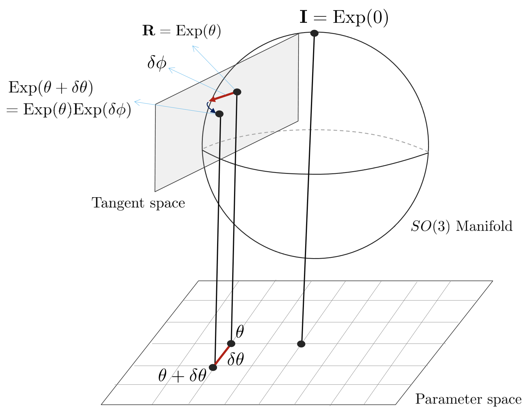
4.3.3 Right Jacobian of SO(3)

임의의 회전행렬 $\mathbf{R}\in SO(3)$와 회전벡터 $\theta \in {\mathbb{R}}^3$가 주어져 있고 $\mathbf{R}=\text{Exp}(\theta )$와 같이 나타낼 수 있다고 하자. 만약 $\theta$ 값이 미세 변화량 $\delta \theta$만큼 변한다고 할 때, 이는 $\mathbf{R}$의 접평면 상에 존재하는 so(3) 원소 $\delta \varphi$로 표현할 수 있다.
$$\begin{array}{}\text{(36)}& \begin{array}{r}\text{Exp}(\theta )\oplus \delta \varphi =\text{Exp}(\theta +\delta \theta )\end{array}\end{array}$$

이는 다음과 같이 나타낼 수 있다.
$$\begin{array}{}\text{(37)}& \begin{array}{r}\text{Exp}(\theta )\cdot \text{Exp}(\delta \varphi )=\text{Exp}(\theta +\delta \theta )\end{array}\end{array}$$

또한, 다음과 같이 나타낼 수 있다.
$$\begin{array}{}\text{(38)}& \begin{array}{r}\delta \varphi =\text{Log}(\text{Exp}(\theta {)}^{-1}\cdot \text{Exp}(\theta +\delta \theta ))=\text{Exp}(\theta +\delta \theta )\ominus \text{Exp}(\theta )\end{array}\end{array}$$

파라미터 공간에서 미세 변화량 $\delta \theta$와에 대한 so(3)에서 미세 변화량 $\delta \varphi$는 다음과 같이 자코비안으로 나타낼 수 있다.
$$\begin{array}{}\text{(39)}& \begin{array}{r}\frac{\partial \delta \varphi }{\partial \delta \theta }=\underset{\delta \theta \to 0}{lim}\frac{\delta \varphi }{\delta \theta }=\underset{\partial \theta \to 0}{lim}\frac{\text{Exp}(\theta +\delta \theta )\ominus \text{Exp}(\theta )}{\delta \theta }\end{array}\end{array}$$

이는 ${\mathbb{R}}^3\mapsto SO(3)$를 만족하는 함수 $f(\theta )=\text{Exp}(\theta )$에 대한 미분인 ($\text{???}$)의 형태를 가진다. 이는 미세변화량 $\delta \varphi$을 기존 SO(3)군의 오른쪽에 곱하는 $\text{Exp}(\theta )\text{Exp}(\delta \varphi )$ 형태를 가지므로 오른 자코비안(right jacobian)이라고 한다.

오른 자코비안은 다음과 같이 정의된다.
$$\begin{array}{}\text{(40)}& \begin{array}{r}{\mathbf{J}}_r\triangleq \frac{\partial \text{Exp}(\theta )}{\partial \theta }\end{array}\end{array}$$

이는 회전 연산자 표기법과 독립적으로 정의할 수 있다. ($\text{???}$)를 사용하여 $\mathbf{R},\mathbf{q}$ 회전 연산장에 대해 정의하면 다음과 같다.
$$\begin{array}{}\text{(41)}& \begin{array}{rl}{\mathbf{J}}_r(\theta )& =\underset{\delta \theta \to 0}{lim}\frac{\text{Exp}(\theta +\delta \theta )\ominus \text{Exp}(\theta )}{\partial \theta }\\ & =\underset{\partial \theta \to 0}{lim}\frac{\text{Log}(\text{Exp}(\theta {)}^{⊺}\text{Exp}(\theta +\delta \theta ))}{\partial \theta }\text{if using }\mathbf{R}\\ & =\underset{\partial \theta \to 0}{lim}\frac{\text{Log}(\text{Exp}(\theta {)}^{\ast }\otimes \text{Exp}(\theta +\delta \theta ))}{\delta \theta }\text{if using }\mathbf{q}\end{array}\end{array}$$

오른 자코비안의 역함수는 다음과 같이 closed form으로 계산할 수 있다. (Chirikjian, 2012, paper 40).
$$\begin{array}{}\text{(42)}& \begin{array}{rl}& {\mathbf{J}}_r(\theta )=\mathbf{I}-\frac{1-\cos \Vert \theta \Vert }{{\Vert \theta \Vert }^2}[\theta {]}_{\times }+\frac{\Vert \theta \Vert -\sin \Vert \theta \Vert }{{\Vert \theta \Vert }^3}[\theta {]}_{\times }^2\\ & {\mathbf{J}}_r^{-1}(\theta )=\mathbf{I}+\frac{1}{2}[\theta {]}_{\times }+(\frac{1}{{\Vert \theta \Vert }^2}-\frac{1+\cos \Vert \theta \Vert }{2\Vert \theta \Vert \sin \Vert \theta \Vert })[\theta {]}_{\times }^2\end{array}\end{array}$$

추가적으로 SO(3)의 오른 자코비안은 미세 변화량 $\delta \theta$에 대해 다음과 같은 성질을 같는다.
$$\begin{array}{}\text{(43)}& \begin{array}{rlrl}& \text{Exp}(\theta +\delta \theta )& & \approx \text{Exp}(\theta )\text{Exp}({\mathbf{J}}_r(\theta )\delta \theta )\\ & \text{Exp}(\theta )\text{Exp}(\delta \theta )& & \approx \text{Exp}(\theta +{\mathbf{J}}_r^{-1}(\theta )\delta \theta )\\ & \text{Log}(\text{Exp}(\theta )\text{Exp}(\delta \theta ))& & \approx \theta +{\mathbf{J}}_r^{-1}(\theta )\delta \theta \end{array}\end{array}$$

4.3.4 Jacobian with respect to the rotation vector

임의의 회전벡터 $\theta$에 대한 회전 ${\mathbf{a}}^{\prime }=\mathbf{R}\{\theta \}\mathbf{a}$은 ${\mathbb{R}}^3\mapsto {\mathbb{R}}^3$를 만족하는 함수이다. 이는 ($\text{???}$)와 같이 나타낼 수 있으며 ($\text{43}$)를 사용하여 다음과 같이 나타낼 수 있다.
$$\begin{array}{}\text{(44)}& \begin{array}{rl}\frac{\partial (\mathbf{q}\otimes \mathbf{a}\otimes {\mathbf{q}}^{\ast })}{\partial \delta \theta }=\frac{\partial (\mathbf{Ra})}{\partial \delta \theta }& =\underset{\partial \theta \to 0}{lim}\frac{\mathbf{R}\{\theta +\delta \theta \}\mathbf{a}-\mathbf{R}\{\theta \}\mathbf{a}}{\delta \theta }\\ & =\underset{\partial \theta \to 0}{lim}\frac{(\mathbf{R}\{\theta \}\text{Exp}({\mathbf{J}}_r(\theta )\partial \theta )-\mathbf{R}\{\theta \})\mathbf{a}}{\delta \theta }\\ & =\underset{\partial \theta \to 0}{lim}\frac{(\mathbf{R}\{\theta \}(\mathbf{I}+[{\mathbf{J}}_r(\theta )\delta \theta {]}_{\times })-\mathbf{R}\{\theta \}\mathbf{a})}{\delta \theta }\\ & =\underset{\partial \theta \to 0}{lim}\frac{\mathbf{R}\{\theta \}[{\mathbf{J}}_r(\theta )\delta \theta {]}_{\times }\mathbf{a}}{\delta \theta }\\ & =\underset{\partial \theta \to 0}{lim}-\frac{\mathbf{R}\{\theta \}[\mathbf{a}{]}_{\times }{\mathbf{J}}_r(\theta )\delta \theta }{\delta \theta }\\ & =-\mathbf{R}\{\theta \}[\mathbf{a}{]}_{\times }{\mathbf{J}}_r(\theta )\end{array}\end{array}$$

이 때, $\mathbf{R}\{\theta \}\triangleq \text{Exp}(\theta )$이다. 이를 정리하면 다음과 같다.
$$\begin{array}{}\text{(45)}& \begin{array}{r}\boxed{{\displaystyle \frac{\partial (\mathbf{q}\otimes \mathbf{a}\otimes {\mathbf{q}}^{\ast })}{\partial \delta \theta }=\frac{\partial (\mathbf{Ra})}{\partial \delta \theta }=-\mathbf{R}\{\theta \}[\mathbf{a}{]}_{\times }{\mathbf{J}}_r(\theta )}}\end{array}\end{array}$$

4.3.5 Jacobians of the rotation composition

SO(3)군의 합성 $\mathbf{P}=\mathbf{Q}\cdot \mathbf{R}$이 주어졌을 때, 이는 쿼터니언 또는 회전행렬의 형태로 다음과 같이 나타낼 수 있다.
$$\begin{array}{}\text{(46)}& \begin{array}{r}\mathbf{p}={\mathbf{q}}_{\theta }\otimes {\mathbf{r}}_{\varphi }\mathbf{P}={\mathbf{Q}}_{\theta }{\mathbf{R}}_{\varphi }\end{array}\end{array}$$

접평면에서 미세 변화량 $\delta \theta ,\delta \varphi$에 대한 $SO(3)\mapsto SO(3)$ 함수의 미분을 ($\text{???}$)을 사용하여 나타내면 다음과 같다.
$$\begin{array}{}\text{(47)}& \begin{array}{rl}\frac{\partial \mathbf{Q}\cdot \mathbf{R}}{\partial \mathbf{Q}}=\frac{\partial {\mathbf{q}}_{\theta }\otimes {\mathbf{r}}_{\varphi }}{\partial \theta }=\frac{{\mathbf{Q}}_{\theta }{\mathbf{R}}_{\varphi }}{\partial \theta }& =\underset{\delta \theta \to 0}{lim}\frac{(({\mathbf{Q}}_{\theta }\oplus \delta \theta ){\mathbf{R}}_{\varphi })\ominus ({\mathbf{Q}}_{\theta }{\mathbf{R}}_{\varphi })}{\delta \theta }\\ & =\underset{\delta \theta \to 0}{lim}\frac{\text{Log}[({\mathbf{Q}}_{\theta }{\mathbf{R}}_{\varphi }{)}^{⊺}({\mathbf{Q}}_{\theta }\text{Exp}(\delta \theta ){\mathbf{R}}_{\varphi })]}{\delta \theta }\\ & =\underset{\delta \theta \to 0}{lim}\frac{\text{Log}[{\mathbf{R}}_{\varphi }^{⊺}\text{Exp}(\delta \theta ){\mathbf{R}}_{\varphi }]}{\delta \theta }\\ & =\underset{\delta \theta \to 0}{lim}\frac{\text{Log}[\text{Exp}({\mathbf{R}}_{\varphi }^{⊺}\delta \theta )]}{\delta \theta }\\ & =\underset{\delta \theta \to 0}{lim}\frac{{\mathbf{R}}_{\varphi }^{⊺}\delta \theta }{\delta \theta }\\ & ={\mathbf{R}}_{\varphi }^{⊺}\end{array}\end{array}$$

$$\begin{array}{}\text{(48)}& \begin{array}{rl}\frac{\partial \mathbf{Q}\cdot \mathbf{R}}{\partial \mathbf{R}}=\frac{\partial {\mathbf{q}}_{\theta }\otimes {\mathbf{r}}_{\varphi }}{\partial \varphi }=\frac{{\mathbf{Q}}_{\theta }{\mathbf{R}}_{\varphi }}{\partial \varphi }& =\underset{\delta \varphi \to 0}{lim}\frac{({\mathbf{Q}}_{\theta }({\mathbf{R}}_{\varphi }\oplus \delta \varphi ))\ominus ({\mathbf{Q}}_{\theta }{\mathbf{R}}_{\varphi })}{\delta \varphi }\\ & =\underset{\delta \varphi \to 0}{lim}\frac{\text{Log}[({\mathbf{Q}}_{\theta }{\mathbf{R}}_{\varphi }{)}^{⊺}({\mathbf{Q}}_{\theta }{\mathbf{R}}_{\varphi }\text{Exp}(\delta \varphi ))]}{\partial \varphi }\\ & =\underset{\delta \varphi \to 0}{lim}\frac{\text{Log}[\text{Exp}(\delta \varphi )]}{\delta \varphi }\\ & =\underset{\delta \varphi \to 0}{lim}\frac{\delta \varphi }{\delta \varphi }\\ & =\mathbf{I}\end{array}\end{array}$$

4.4 Perturbations, uncertainties, noise

4.4.1 Local perturbations

섭동 쿼터니언 (perturbed quaternion) $\tilde{\mathbf{q}}$는 원래 섭동하지 않은 쿼터니언 (unperturbed quaternion) $\mathbf{q}$과 작은 로컬 섭동 (small local perturbation) $\mathrm{\Delta }{\mathbf{q}}_{\mathcal{L}}$의 조합으로 나타낼 수 있다. 본 페이지에서는 Hamilton 표기법을 사용하기 때문에 기존 원소 오른쪽에 로컬 섭동을 곱함으로써 나타낼 수 있다. 이는 회전행렬 형태로도 나타낼 수 있다.
$$\begin{array}{}\text{(49)}& \tilde{\mathbf{q}}=\mathbf{q}\otimes \mathrm{\Delta }{\mathbf{q}}_{\mathcal{L}}\tilde{\mathbf{R}}=\mathbf{R}\mathrm{\Delta }{\mathbf{R}}_{\mathcal{L}}\end{array}$$

또한, 로컬 섭동 $\mathrm{\Delta }{\mathbf{q}}_{\mathcal{L}},\mathrm{\Delta }{\mathbf{R}}_{\mathcal{L}}$은 회전벡터의 변화량 $\mathrm{\Delta }{\mathit{\varphi }}_{\mathcal{L}}=\mathbf{u}\mathrm{\Delta }{\varphi }_{\mathcal{L}}$의 exponential map을 사용하여 쉽게 구할 수 있다.
$$\begin{array}{}\text{(50)}& {\tilde{\mathbf{q}}}_{\mathcal{L}}={\mathbf{q}}_{\mathcal{L}}\otimes \text{Exp}(\mathrm{\Delta }{\mathit{\varphi }}_{\mathcal{L}}){\tilde{\mathbf{R}}}_{\mathcal{L}}={\mathbf{R}}_{\mathcal{L}}\cdot \text{Exp}(\mathrm{\Delta }{\mathit{\varphi }}_{\mathcal{L}})\end{array}$$

위 식을 로컬 섭동을 기준으로 정리하면 다음과 같다.
$$\begin{array}{}\text{(51)}& \mathrm{\Delta }{\mathit{\varphi }}_{\mathcal{L}}=\text{Log}({\mathbf{q}}_{\mathcal{L}}^{\ast }\otimes {\tilde{\mathbf{q}}}_{\mathcal{L}})=\text{Log}({\mathbf{R}}_{\mathcal{L}}^{⊺}\cdot {\tilde{\mathbf{R}}}_{\mathcal{L}})\end{array}$$

만약 $\mathrm{\Delta }{\mathit{\varphi }}_{\mathcal{L}}$ 값이 충분히 작으면 쿼터니언과 회전행렬은 ($\text{???}$), ($\text{???}$)의 테일러 전개를 통해 선형적으로 표현할 수 있다.
$$\begin{array}{}\text{(52)}& \mathrm{\Delta }{\mathbf{q}}_{\mathcal{L}}\approx \left[\begin{array}{c}1\\ \frac{1}{2}\mathrm{\Delta }{\mathit{\varphi }}_{\mathcal{L}}\end{array}\right]\mathrm{\Delta }{\mathbf{R}}_{\mathcal{L}}\approx \mathbf{I}+[\mathrm{\Delta }{\mathit{\varphi }}_{\mathcal{L}}{]}_{\times }\end{array}$$

작은 회전량 $\mathrm{\Delta }{\varphi }_{\mathcal{L}}$에 대하여 $\cos (\frac{1}{2}\mathrm{\Delta }{\varphi }_{\mathcal{L}})\approx 1$이고 $\mathbf{u}\sin (\frac{1}{2}\mathrm{\Delta }{\varphi }_{\mathcal{L}})\approx \mathbf{u}\frac{1}{2}\mathrm{\Delta }{\varphi }_{\mathcal{L}}=\frac{1}{2}\mathrm{\Delta }{\mathit{\varphi }}_{\mathcal{L}}$이므로 위 쿼터니언 식이 성립한다. 이와 같이 회전의 섭동(perturbations)은 SO(3) 원소의 접평면인 so(3) 벡터 공간 $\mathrm{\Delta }{\mathit{\varphi }}_{\mathcal{L}}$으로 모델링 할 수 있다. 이는 회전 섭동의 공분산 행렬을 벡터 공간에 대한 $3\times 3$ 행렬로 표현할 수 있는 등 여러가지 이점이 있다.

4.4.2 Global perturbations

다음으로 전역적으로 정의된(globally-defined) 섭동을 생각해볼 수 있다. Hamilton 표기법에서 기존 원소 왼쪽에 곱함으로써 나타낼 수 있다.
$$\begin{array}{}\text{(53)}& {\tilde{\mathbf{q}}}_{\mathcal{G}}=\text{Exp}(\mathrm{\Delta }{\mathit{\varphi }}_{\mathcal{G}})\otimes {\mathbf{q}}_{\mathcal{G}}\tilde{\mathbf{R}}=\text{Exp}(\mathrm{\Delta }{\mathit{\varphi }}_{\mathcal{G}})\cdot {\mathbf{R}}_{\mathcal{G}}\end{array}$$

전역 섭동은 다음과 같이 나타낼 수 있다.
$$\begin{array}{}\text{(54)}& \mathrm{\Delta }{\mathit{\varphi }}_{\mathcal{G}}=\text{Log}({\tilde{\mathbf{q}}}_{\mathcal{G}}\otimes {\mathbf{q}}_{\mathcal{G}}^{\ast })=\text{Log}(\tilde{\mathbf{R}}\cdot {\mathbf{R}}_{\mathcal{G}}^{⊺})\end{array}$$

4.5 Time derivatives

회전의 로컬 섭동(local perturbations)을 벡터로 표현함으로써 이에 대한 시간미분을 쉽게 계산할 수 있는 이점이 있다. 시간에 따른 쿼터니언 함수를 $\mathbf{q}=\mathbf{q}(t)$라고 하고 해당 함수의 섭동을 $\tilde{\mathbf{q}}=\mathbf{q}(t+\mathrm{\Delta }t)$라고 하면, 이에 대한 시간 미분은 다음과 같다.
$$\begin{array}{}\text{(55)}& \frac{d\mathbf{q}(t)}{dt}\triangleq \underset{\mathrm{\Delta }t\to 0}{lim}\frac{\mathbf{q}(t+\mathrm{\Delta }t)-\mathbf{q}(t)}{\mathrm{\Delta }t}\end{array}$$

또한, 로컬 각속도 ${\mathit{\omega }}_{\mathcal{L}}$을 다음과 같이 정의할 수 있다.
$$\begin{array}{}\text{(56)}& {\mathit{\omega }}_{\mathcal{L}}(t)\triangleq \frac{d{\mathit{\varphi }}_{\mathcal{L}}}{dt}\triangleq \frac{\mathrm{\Delta }{\mathit{\varphi }}_{\mathcal{L}}}{\mathrm{\Delta }t}\end{array}$$

이 때, $\mathrm{\Delta }{\mathit{\varphi }}_{\mathcal{L}}$은 $\mathbf{q}$의 접평면 상에 존재하는 로컬 각속도 섭동(local angular perturbation)을 의미한다.

쿼터니언의 시간 미분은 다음과 같이 유도할 수 있다.
$$\begin{array}{}\text{(57)}& \begin{array}{rl}\dot{\mathbf{q}}& \triangleq \underset{\mathrm{\Delta }t\to 0}{lim}\frac{\mathbf{q}(t+\mathrm{\Delta }t)-\mathbf{q}(t)}{\mathrm{\Delta }t}\\ & =\underset{\mathrm{\Delta }t\to 0}{lim}\frac{\mathbf{q}\otimes \mathrm{\Delta }{\mathbf{q}}_{\mathcal{L}}-\mathbf{q}}{\mathrm{\Delta }t}\\ & =\underset{\mathrm{\Delta }t\to 0}{lim}\frac{\mathbf{q}\otimes (\left[\begin{array}{c}1\\ \mathrm{\Delta }{\mathit{\varphi }}_{\mathcal{L}}/2\end{array}\right]-\left[\begin{array}{c}1\\ 0\end{array}\right])}{\mathrm{\Delta }t}\\ & =\underset{\mathrm{\Delta }t\to 0}{lim}\frac{\mathbf{q}\otimes \left[\begin{array}{c}0\\ \mathrm{\Delta }{\mathit{\varphi }}_{\mathcal{L}}/2\end{array}\right]}{\mathrm{\Delta }t}\\ & =\frac{1}{2}\mathbf{q}\otimes \left[\begin{array}{c}0\\ {\mathit{\omega }}_{\mathcal{L}}\end{array}\right]\end{array}\end{array}$$

표기의 편의를 위해 다음과 같이 정의한다.
$$\begin{array}{}\text{(58)}& \mathrm{\Omega }(\mathit{\omega })\triangleq [\mathit{\omega }{]}_R=\left[\begin{array}{cc}0& -{\mathit{\omega }}^{⊺}\\ \mathit{\omega }& -[\mathit{\omega }{]}_{\times }\end{array}\right]=\left[\begin{array}{cccc}0& -{\omega }_x& -{\omega }_y& -{\omega }_z\\ {\omega }_x& 0& {\omega }_z& -{\omega }_y\\ {\omega }_y& -{\omega }_z& 0& {\omega }_x\\ {\omega }_z& {\omega }_y& -{\omega }_x& 0\end{array}\right]\end{array}$$

최종적으로 ($\text{???}$), ($\text{57}$)로부터 다음을 얻을 수 있다.
$$\begin{array}{}\text{(59)}& \boxed{{\displaystyle \dot{\mathbf{q}}=\frac{1}{2}\mathrm{\Omega }({\mathit{\omega }}_{\mathcal{L}})\mathbf{q}=\frac{1}{2}\mathbf{q}\otimes {\mathit{\omega }}_{\mathcal{L}}\dot{\mathbf{R}}=\mathbf{R}[{\mathit{\omega }}_{\mathcal{L}}{]}_{\times }}}\end{array}$$

이는 ($\text{???}$), ($\text{???}$)을 SO(3) 프레임워크로 확장한 표현이다. 위 식은 $\mathbf{q},\mathbf{R}$의 시간미분을 이에 대한 각속도 ${\mathit{\omega }}_{\mathcal{L}}$로 표현할 수 있음을 의미한다.

($\text{59}$)은 각속도가 로컬 좌표계에서 표현되었을 때 미분 값을 의미한다. 이와 달리 전역 섭동(global perturbations)에 대한 시간미분은 ($\text{57}$)를 사용하여 다음과 같이 나타낼 수 있다.
$$\begin{array}{}\text{(60)}& \boxed{{\displaystyle \dot{\mathbf{q}}=\frac{1}{2}{\mathit{\omega }}_{\mathcal{G}}\otimes \mathbf{q}\dot{\mathbf{R}}=[{\mathit{\omega }}_{\mathcal{G}}{]}_{\times }\mathbf{R}}}\end{array}$$

이 때, ${\mathit{\omega }}_{\mathcal{G}}\triangleq \frac{d{\mathit{\varphi }}_{\mathcal{G}}(t)}{dt}$은 전역 프레임에서 바라본 각속도 벡터를 의미한다. 따라서 ($\text{60}$)은 전역 좌표계에서 각속도를 나타내었을 때 미분 값을 의미한다.

4.5.1 Global-to-local relations

전역 미분값과 지역(=로컬) 미분값의 관계는 다음과 같다.
$$\begin{array}{}\text{(61)}& \frac{1}{2}{\mathit{\omega }}_{\mathcal{G}}\otimes \mathbf{q}=\dot{\mathbf{q}}=\frac{1}{2}\mathbf{q}\otimes {\mathit{\omega }}_{\mathcal{L}}\end{array}$$

이를 정리하면 다음과 같다.
$$\begin{array}{}\text{(62)}& {\mathit{\omega }}_{\mathcal{G}}=\mathbf{q}\otimes {\mathit{\omega }}_{\mathcal{L}}\otimes {\mathbf{q}}^{\ast }=\mathbf{R}{\mathit{\omega }}_{\mathcal{L}}\end{array}$$

충분히 작은 시간 변화량 $\mathrm{\Delta }t$에 대해 $\mathrm{\Delta }{\mathit{\varphi }}_R\approx \mathit{\omega }\mathrm{\Delta }t$이라고 하면 다음과 같다.
$$\begin{array}{}\text{(63)}& \mathrm{\Delta }{\mathit{\varphi }}_{\mathcal{G}}=\mathbf{q}\otimes \mathrm{\Delta }{\mathit{\varphi }}_{\mathcal{L}}\otimes {\mathbf{q}}^{\ast }=\mathbf{R}\mathrm{\Delta }{\mathit{\varphi }}_{\mathcal{L}}\end{array}$$

이는 각속도 벡터 $\mathit{\omega }$와 작은 각도 섭동 $\mathrm{\Delta }\mathit{\varphi }$를 쿼터니언과 회전행렬을 통해 일반 벡터와 같이 좌표계 변환을 수행할 수 있음을 의미한다. 이는 $\mathit{\omega }=\mathbf{u}\omega$와 $\mathrm{\Delta }\mathit{\varphi }=\mathbf{u}\mathrm{\Delta }\varphi$에서 회전축 $\mathbf{u}$에 대해서도 동일하게 적용된다.
$$\begin{array}{}\text{(64)}& {\mathbf{u}}_{\mathcal{G}}=\mathbf{q}\otimes {\mathbf{u}}_{\mathcal{L}}\otimes {\mathbf{q}}^{\ast }=\mathbf{R}{\mathbf{u}}_{\mathcal{L}}\end{array}$$

4.5.2 Time-derivative of the quaternion product

회전 곱셈 연산자에 대한 시간 미분은 다음과 같다.
$$\begin{array}{}\text{(65)}& \dot{{\mathbf{q}}_1\otimes {\mathbf{q}}_2}={\dot{\mathbf{q}}}_1\otimes {\mathbf{q}}_2+{\mathbf{q}}_1\otimes {\dot{\mathbf{q}}}_2,\dot{(}{\mathbf{R}}_1{\mathbf{R}}_2)={\dot{\mathbf{R}}}_1{\mathbf{R}}_2+{\mathbf{R}}_1{\dot{\mathbf{R}}}_2\end{array}$$

회전의 곱셈 연산자는 교환법칙이 성립하지 않기 때문에, 순서를 엄격하게 지켜서 표기해야 한다. 이는 즉, $\dot{{\mathbf{q}}_2}\ne 2\mathbf{q}\otimes \dot{\mathbf{q}}$임을 의미한다. 동일한 쿼터니언의 곱에 대한 미분은 다음과 같다.
$$\begin{array}{}\text{(66)}& \dot{{\mathbf{q}}^2}=\dot{\mathbf{q}}\otimes \mathbf{q}+\mathbf{q}\otimes \dot{\mathbf{q}}\end{array}$$

4.5.3 Other useful expressions with the derivatives

로컬 회전에 대한 미분을 정리하면 ${\mathit{\omega }}_{\mathcal{L}}$를 다음과 같이 나타낼 수 있다.
$$\begin{array}{}\text{(67)}& {\mathit{\omega }}_{\mathcal{L}}=2{\mathbf{q}}^{\ast }\otimes \dot{\mathbf{q}},[{\mathit{\omega }}_{\mathcal{L}}{]}_{\times }={\mathbf{R}}^{⊺}\dot{\mathbf{R}}\end{array}$$

전역 회전에 대한 미분을 정리하면 ${\mathit{\omega }}_{\mathcal{G}}$를 다음과 같이 나타낼 수 있다.
$$\begin{array}{}\text{(68)}& {\mathit{\omega }}_{\mathcal{G}}=2\dot{\mathbf{q}}\otimes {\mathbf{q}}^{\ast },[{\mathit{\omega }}_{\mathcal{G}}{]}_{\times }=\dot{\mathbf{R}}{\mathbf{R}}^{⊺}\end{array}$$

4.6 Time-integration of rotation rates

시간에 따른 쿼터니언 회전 변화는 이전 섹션에서 유도했던 ($\text{59}$)과 ($\text{60}$)을 적분함으로써 구할 수 있다. 이 때, 각속도가 로컬 각속도인 경우에는 ($\text{59}$)를 사용하고 전역 각속도인 경우에는 ($\text{60}$)를 사용한다. SLAM과 같은 문제는 일반적으로 로봇에 부착된 로컬 센서가 각속도를 측정하여 로컬 각속도 측정값 $\mathit{\omega }(t_n)$, $t_n=n\mathrm{\Delta }t$을 제공한다. 본 섹션에서는 이러한 로컬 케이스에 대한 적분 내용만 다룬다. ($\text{59}$)은 다음과 같다.
$$\begin{array}{}\text{(69)}& \dot{\mathbf{q}}(t)=\frac{1}{2}\mathbf{q}(t)\otimes \mathit{\omega }(t)\end{array}$$

실제 센서 데이터는 이산시간(discrete time) 입력으로 들어오기 때문에 위 식을 바로 사용할 수 없다. 따라서 여러 가지 수치적분 방법들이 개발되었는데 본 문서에서는 0차, 1차 수치적분(zeroth, first order integration) 방법에 대해서 설명한다. 두 방법은 모두 $\mathbf{q}(t_n+\mathrm{\Delta }t)$를 $t=t_n$에 대한 테일러 급수로 근사화하는 방법이다. $\mathbf{q}\triangleq \mathbf{q}(t)$, ${\mathbf{q}}_n=\mathbf{q}(t_n)$과 같이 간단하게 표기한다. 시간함수의 테일러 급수는 다음과 같다.
$$\begin{array}{}\text{(70)}& {\mathbf{q}}_{n+1}={\mathbf{q}}_n+{\dot{\mathbf{q}}}_n\mathrm{\Delta }t+\frac{1}{2!}{\ddot{\mathbf{q}}}_n\mathrm{\Delta }{t}^2+\frac{1}{3!}{\stackrel{⃛}{\mathbf{q}}}_n\mathrm{\Delta }{t}^3\frac{1}{4!}{\stackrel{⃜}{\mathbf{q}}}_n\mathrm{\Delta }{t}^4+\cdots \end{array}$$

쿼터니언 미분 값은 ($\text{???}$)를 통해 구할 수 있다. 이 때, 각속도의 두 번 미분값인 $\ddot{\mathit{\omega }}=0$이다.
$$\begin{array}{}\text{(71)}& \begin{array}{rl}& \dot{\mathbf{q}}=\frac{1}{2}{\mathbf{q}}_n{\mathit{\omega }}_n\\ & {\ddot{\mathbf{q}}}_n=\frac{1}{2^2}{\mathbf{q}}_n{\mathit{\omega }}_n^2+\frac{1}{2}{\mathbf{q}}_n{\dot{\mathit{\omega }}}_n\\ & {\stackrel{⃛}{\mathbf{q}}}_n=\frac{1}{2^3}{\mathit{\omega }}_n^3+\frac{1}{4}{\mathbf{q}}_n\dot{\mathit{\omega }}{\mathit{\omega }}_n+\frac{1}{2}\mathbf{q}{\mathit{\omega }}_n\dot{\mathit{\omega }}\\ & {\mathbf{q}}_n^{(i\ge 4)}=\frac{1}{2^i}{\mathbf{q}}_n{\mathit{\omega }}_n^i+\cdots \end{array}\end{array}$$

위 식은 표기의 편의 상 $\otimes$ 연산자를 생략하였다. 실제 연산에서는 모든 $\mathit{\omega }$의 지수승들이 쿼터니언 곱으로 곱해져야한다.

4.6.1 Zeroth order integration

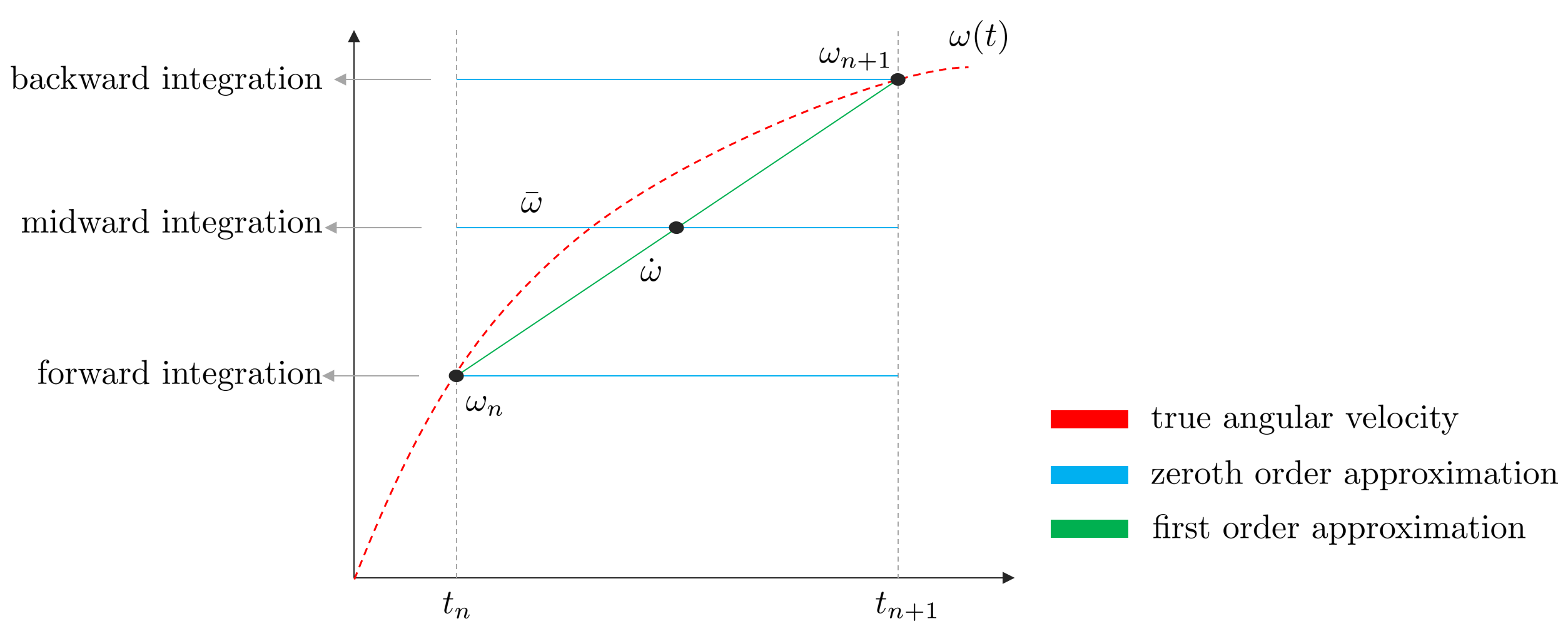
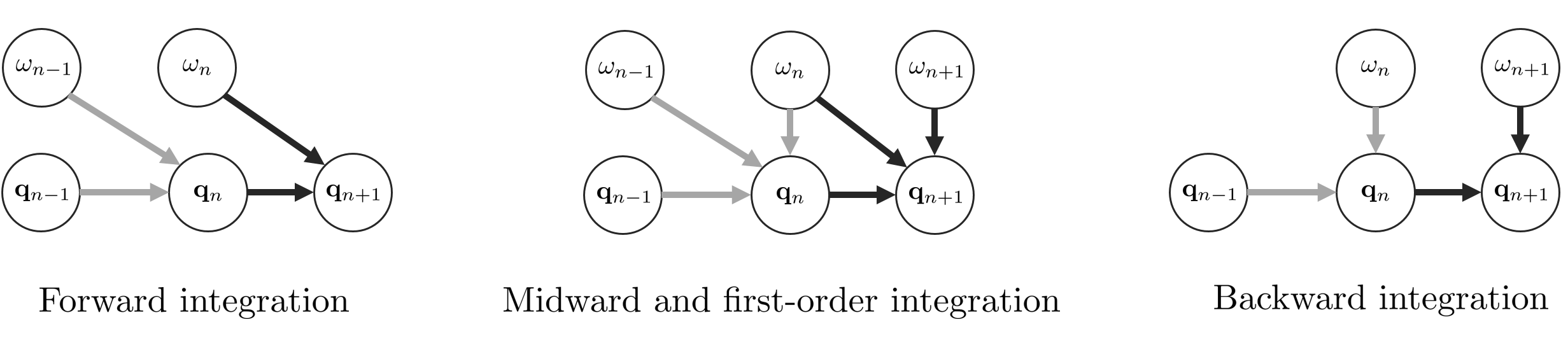
Forward integration 각속도 ${\mathit{\omega }}_n$가 시간 $[t_n,t_{n+1}]$ 구간동안 일정하다고 가정하여 적분하는 방법이다. 이 때, $\dot{\mathit{\omega }}=0$이 된다. ($\text{70}$)을 다시 나타내면 다음과 같다.
$$\begin{array}{}\text{(72)}& {\mathbf{q}}_{n+1}={\mathbf{q}}_n\otimes (1+\frac{1}{2}{\mathit{\omega }}_n\mathrm{\Delta }t+\frac{1}{2!}(\frac{1}{2}{\mathit{\omega }}_n\mathrm{\Delta }t{)}^2+\frac{1}{3!}(\frac{1}{2}{\mathit{\omega }}_n\mathrm{\Delta }t{)}^3+\cdots )\end{array}$$

위 식에서 뒷 부분은 $e^{\mathit{\omega }\mathrm{\Delta }t/2}$의 테일러 급수를 ($\text{???}$)과 같이 펼쳐놓은 형태이다. ($\text{???}$)로부터 이러한 exponential term은 쿼터니언으로 변환될 수 있다.
$$\begin{array}{}\text{(73)}& e^{\mathit{\omega }\mathrm{\Delta }t/2}=\text{Exp}(\mathit{\omega }\mathrm{\Delta }t)=\mathbf{q}\{\mathit{\omega }\mathrm{\Delta }t\}=\left[\begin{array}{c}\cos (\Vert \mathit{\omega }\Vert \mathrm{\Delta }t/2)\\ \frac{\mathit{\omega }}{\Vert \mathit{\omega }\Vert }\sin (\Vert \mathit{\omega }\Vert \mathrm{\Delta }t/2)\end{array}\right]\end{array}$$

따라서 다음 식이 유도된다.
$$\begin{array}{}\text{(74)}& \boxed{{\displaystyle {\mathbf{q}}_{n+1}={\mathbf{q}}_n\otimes \mathbf{q}\{\mathit{\omega }\mathrm{\Delta }t\}}}\end{array}$$

Backward integration $\mathrm{\Delta }t$의 맨 마지막 구간 $t_{n+1}$의 각속도인 ${\mathit{\omega }}_{n+1}$을 사용하여 적분하는 방법이다. 이는 $t_{n+1}$에서 ${\mathbf{q}}_n$의 테일러 급수를 전개하는 것과 유사하다.
$$\begin{array}{}\text{(75)}& {\mathbf{q}}_{n+1}\approx {\mathbf{q}}_n\otimes \mathbf{q}\{{\mathit{\omega }}_{n+1}\mathrm{\Delta }t\}\end{array}$$

위 방법은 마지막으로 측정된 각속도 ${\mathit{\omega }}_{n+1}$을 기준으로 적분하는 성질로 인해 실시간 처리가 중요한 로보틱스 분야 등에서 주로 사용하는 방법이다. 시간 스텝을 한 단계 앞서서 표현하면 다음과 같다.
$$\begin{array}{}\text{(76)}& \boxed{{\displaystyle {\mathbf{q}}_n={\mathbf{q}}_{n-1}\otimes \mathbf{q}\{{\mathit{\omega }}_n\mathrm{\Delta }t\}}}\end{array}$$

Midward integration 각속도 $\mathit{\omega }$를 처음과 끝의 중간으로 설정하여 적분하는 방법이다.
$$\begin{array}{}\text{(77)}& \overline{\mathit{\omega }}=\frac{{\mathit{\omega }}_{n+1}+{\mathit{\omega }}_n}{2}\end{array}$$

이를 통해 다음 식을 구할 수 있다.
$$\begin{array}{}\text{(78)}& \boxed{{\displaystyle {\mathbf{q}}_{n+1}={\mathbf{q}}_n\otimes \mathbf{q}\{\overline{\mathit{\omega }}\mathrm{\Delta }t\}}}\end{array}$$

4.6.2 First order integration

1차 수치적분은 각속도 $\mathit{\omega }(t)$를 1차 함수(직선)으로 근사하는 적분이다. 테일러 급수 항에서 2차 이상의 항은 전부 0으로 간주한다.
$$\begin{array}{}\text{(79)}& \begin{array}{rl}& \dot{\mathit{\omega }}=\frac{{\mathit{\omega }}_{n+1}-{\mathit{\omega }}_n}{\mathrm{\Delta }t}\\ & \ddot{\mathit{\omega }}=\stackrel{⃛}{\mathit{\omega }}=\cdots =0\end{array}\end{array}$$

이를 사용하여 중간값 $\overline{\mathit{\omega }}$를 다음과 같이 나타낼 수 있다.
$$\begin{array}{}\text{(80)}& \overline{\mathit{\omega }}={\mathit{\omega }}_n+\frac{1}{2}\dot{\mathit{\omega }}\mathrm{\Delta }t\end{array}$$

또한 각속도의 지수승 ${\mathit{\omega }}_n^k$를 다음과 같이 나타낼 수 있다.
$$\begin{array}{}\text{(81)}& \begin{array}{rl}& {\mathit{\omega }}_n=\overline{\mathit{\omega }}-\frac{1}{2}\dot{\mathit{\omega }}\mathrm{\Delta }t\\ & {\mathit{\omega }}_n^2={\overline{\mathit{\omega }}}^2-\frac{1}{2}\overline{\mathit{\omega }}\dot{\mathit{\omega }}\mathrm{\Delta }t-\frac{1}{2}\dot{\mathit{\omega }}\overline{\mathit{\omega }}\mathrm{\Delta }t+\frac{1}{4}{\dot{\mathit{\omega }}}^2\mathrm{\Delta }{t}^2\\ & {\mathit{\omega }}_n^3={\overline{\mathit{\omega }}}^3-\frac{3}{2}{\overline{\mathit{\omega }}}^2\dot{\mathit{\omega }}\mathrm{\Delta }t+\frac{3}{4}\overline{\mathit{\omega }}{\dot{\mathit{\omega }}}^2\mathrm{\Delta }{t}^2+\frac{1}{8}{\dot{\mathit{\omega }}}^3\mathrm{\Delta }{t}^3\\ & {\mathit{\omega }}_n^4={\overline{\mathit{\omega }}}^4+\cdots \end{array}\end{array}$$

이를 쿼터니언 테일러 급수 식에 넣고 정리하면 다음과 같다. 식이 복잡하므로 $\otimes$ 연산자는 생략한다.
$$\begin{array}{}\text{(82)}& \begin{array}{rl}{\mathbf{q}}_{n+1}& =\mathbf{q}(1+\frac{1}{2}\overline{\mathit{\omega }}\mathrm{\Delta }t+\frac{1}{2!}(\frac{1}{2}\overline{\mathit{\omega }}\mathrm{\Delta }t{)}^2+\frac{1}{3!}(\frac{1}{2}\overline{\mathit{\omega }}\mathrm{\Delta }t{)}^3+\cdots )\\ & +\mathbf{q}(-\frac{1}{4}\dot{\mathit{\omega }}+\frac{1}{4}\dot{\mathit{\omega }})\mathrm{\Delta }{t}^2\\ & +\mathbf{q}(-\frac{1}{16}\overline{\mathit{\omega }}\dot{\mathit{\omega }}-\frac{1}{16}\dot{\mathit{\omega }}\overline{\mathit{\omega }}+\frac{1}{24}\dot{\mathit{\omega }}\overline{\mathit{\omega }}+\frac{1}{12}\overline{\mathit{\omega }}\dot{\mathit{\omega }})\mathrm{\Delta }{t}^3\\ & +\mathbf{q}(\cdots )\mathrm{\Delta }{t}^4+\cdots \end{array}\end{array}$$

위 식에서 첫번째 줄은 $e^{\overline{\mathit{\omega }}\mathrm{\Delta }t}=\mathbf{q}\{\overline{\mathit{\omega }}\mathrm{\Delta }t\}$인 것을 알 수 있다. 두번째 줄은 소거되어 없어지고 네번째 줄 이상은 고차항이므로 무시하면 다음과 같이 비교적 간단하게 나타낼 수 있다. $\otimes$ 연산자를 다시 표기하면 다음과 같다.
$$\begin{array}{}\text{(83)}& {\mathbf{q}}_{n+1}={\mathbf{q}}_n\otimes \mathbf{q}\{\overline{\mathit{\omega }}\mathrm{\Delta }t\}+\frac{\mathrm{\Delta }{t}^3}{48}{\mathbf{q}}_n\otimes (\overline{\mathit{\omega }}\otimes \dot{\mathit{\omega }}-\dot{\mathit{\omega }}\otimes \overline{\mathit{\omega }})+\cdots \end{array}$$

$\overline{\mathit{\omega }},\dot{\mathit{\omega }}$를 ($\text{77}$), ($\text{79}$) 같이 풀어서 쓰면 다음과 같다.
$$\begin{array}{}\text{(84)}& {\mathbf{q}}_{n+1}={\mathbf{q}}_n\otimes \mathbf{q}\{\overline{\mathit{\omega }}\mathrm{\Delta }t\}+\frac{\mathrm{\Delta }{t}^3}{48}{\mathbf{q}}_n\otimes ({\mathit{\omega }}_n\otimes {\mathit{\omega }}_{n+1}-{\mathit{\omega }}_{n+1}\otimes {\mathit{\omega }}_n)+\cdots \end{array}$$

위 식은 (Trawny and Roumelotis, 2005)의 결과와 동일하지만 Hamilton 쿼터니언 표기법을 사용하는점이 다르다. 최종적으로 ${\mathbf{a}}_v\otimes {\mathbf{b}}_v-{\mathbf{b}}_v\otimes {\mathbf{a}}_v=2{\mathbf{a}}_v\times {\mathbf{b}}_v$를 사용하여 다음과 같이 나타낼 수 있다.
$$\begin{array}{}\text{(85)}& \boxed{{\displaystyle {\mathbf{q}}_{n+1}\approx {\mathbf{q}}_n\otimes (\mathbf{q}\{\overline{\mathit{\omega }}\mathrm{\Delta }t\}+\frac{\mathrm{\Delta }{t}^2}{24}\left[\begin{array}{c}0\\ {\mathit{\omega }}_n\times {\mathit{\omega }}_{n+1}\end{array}\right])}}\end{array}$$

위 식에서 앞에 있는 항은 midward 1차 수치적분과 동일한 형태 ($\text{78}$)를 띈다는 것을 알 수 있고 뒤에 있는 항은 ${\mathit{\omega }}_n$과 ${\mathit{\omega }}_{n+1}$이 서로 collinear한 경우 소거되는 2차항인 것을 알 수 있다. collinear하다는 의미는 $[t_n,t_{n+1}]$ 구간에서 회전축이 변하지 않는다는 것을 의미한다.

Case of fixed rotation axis 회전축 $\mathbf{u}$을 중심으로 $\omega$만큼 회전하는 각속도의 시간함수를 $\mathit{\omega }(t)=\mathbf{u}(t)\omega (t)$라고 하자. 만약 $\mathbf{u}$가 일정하다고 하면 $\mathbf{u}(t)=\mathbf{u}$이고 ${\mathit{\omega }}_n\times {\mathit{\omega }}_{n+1}=0$을 만족한다. 이를 통해 위 1차 수치적분 공식을 나타내면 다음과 같다.
$$\begin{array}{}\text{(86)}& {\mathbf{q}}_{n+1}={\mathbf{q}}_n\otimes \mathbf{q}\{\mathbf{u}\overline{\omega }\mathrm{\Delta }t\}\end{array}$$

또한, 회전축이 고정되어 있으면 미세 변화량에 대해 쿼터니언의 교환법칙이 성립한다.
$$\begin{array}{}\text{(87)}& e^{\mathbf{u}{\omega }_1\delta t_1}{e}^{\mathbf{u}{\omega }_2\delta t_2}=e^{\mathbf{u}{\omega }_2\delta t_2}{e}^{\mathbf{u}{\omega }_1\delta t_1}=e^{\mathbf{u}({\omega }_1\delta t_1+{\omega }_2\delta t_2)}\end{array}$$

또한 다음 공식이 성립한다.
$$\begin{array}{}\text{(88)}& \begin{array}{rl}{\mathbf{q}}_{n+1}& =\mathbf{q}\otimes e^{\frac{\mathbf{u}}{2}{\int }_{t_n}^{t_{n+1}}\omega (t)\delta t}\\ & ={\mathbf{q}}_n\otimes e^{\mathbf{u}\mathrm{\Delta }{\theta }_n/2}\\ & ={\mathbf{q}}_n\otimes \mathbf{q}\{\mathbf{u}\mathrm{\Delta }{\theta }_n\}\end{array}\end{array}$$

이 때, $\mathrm{\Delta }{\theta }_n={\int }_{t_n}^{t_{n+1}}\omega (t)dt\in \mathbb{R}$은 $[t_n,t_{n+1}]$ 시간동안 최종적으로 돌아간 각도를 의미한다.

Case of varying rotation axis 회전축이 고정되어 있지 않다면 ${\mathit{\omega }}_n\times {\mathit{\omega }}_{n+1}\ne 0$를 만족하고 이에 따라 ($\text{85}$)에서 뒤에 있는 2차항은 사라지지 않고 영향을 준다. 실제 IMU를 사용할 때는 이를 고려하여 샘플링 시간을 $\mathrm{\Delta }t\le 0.01s$로 설정한다. 샘플링 시간이 매우 짧으므로 관성에 의해 ${\mathit{\omega }}_n\simeq {\mathit{\omega }}_{n+1}$이 만족하고 2차항 값은 일반적으로 ${10}^{-6}{\Vert \mathit{\omega }\Vert }^2$보다 작아지게 된다. 2차항 이상의 값은 그보다 더 작아지므로 무시 가능한 값이 된다.

실제 활용 예시에서, 0차 수치적분은 단위 쿼터니언(unit quaternion)을 유지하는 반면에 1차 수치적분은 앞서 말한 2차항의 값으로 인해 단위 쿼터니언 제약조건이 꺠질 수 있다. 따라서 1차 수치적분을 사용한다면 주기적으로 단위 쿼터니언 제약조건을 업데이트 해야 한다 ($\mathbf{q}\leftarrow \mathbf{q}/\Vert \mathbf{q}\Vert$). 만약 회전축이 고정되어 있다는 조건이 유지될 때만 제약조건 업데이트를 고려하지 않아도 된다.

References

[1] Sola, Joan. "Quaternion kinematics for the error-state Kalman filter." arXiv preprint arXiv:1711.02508 (2017).