Quaternion kinematics for the error-state Kalman filter 내용 정리 Part 1

본 포스트는 Joan Solà의 "Quaternion kinematics for the error-state Kalam filter (2017)" 페이퍼를 정리한 포스트이다. 이는 Quaternion과 SO(3) 군, Error-state Kalman filter 모델링에 대해 자세히 나와있어서 SLAM을 공부할 때 이론적인 부분을 참고하면 좋은 페이퍼이다.

1 Quaternion Definition and properties

1.1 Definition of quaternion

두 개의 복소수 $A=a+bi,C=c+di$가 주어졌을 때 이를 $Q=A+Cj$와 같이 구성하고 $k\triangleq ij$로 정의하면 $Q$는 쿼터니언 공간 $\mathbb{H}$ 안에 존재하는 수가 된다.
$$\begin{array}{}\text{(1)}& \begin{array}{r}Q=a+bi+cj+dk\in \mathbb{H}\end{array}\end{array}$$

이 때, $a,b,c,d\in \mathbb{R}$이고 $\{i,j,k\}$는 다음과 같이 정의된 3개의 허수를 의미한다.
$$\begin{array}{}\text{(2)}& \begin{array}{r}{i}^2=j^2=k^2=ijk=-1\end{array}\end{array}$$

이는 다음과 같은 성질을 만족한다.
$$\begin{array}{}\text{(3)}& \begin{array}{r}ij=-ji=k,jk=-kj=i,ki=-ik=j\end{array}\end{array}$$

임의의 쿼터니언 $Q$는 복소수가 0일 때도 쿼터니언을 만족해야하므로 다음과 같은 수 또한 모두 쿼터니언이다.
$$\begin{array}{}\text{(4)}& \begin{array}{r}Q=a\in \mathbb{R}\subset \mathbb{H},Q=bi\in \mathbb{I}\subset \mathbb{H},Q=a+bi\in \mathbb{Z}\subset \mathbb{H}\end{array}\end{array}$$

또한 실수가 0일 때도 쿼터니언을 만족해야 하는데 이때는 특별히 복소수 $\{i,j,k\}$만으로 구성된 순수 쿼터니언(pure quaternion)이라고 한다. 이는 순수 쿼터니언 공간 ${\mathbb{H}}_p=\text{Im}(\mathbb{H})$에 존재한다고 정의한다.
$$\begin{array}{}\text{(5)}& \begin{array}{r}Q=bi+cj+dk\in {\mathbb{H}}_p\subset \mathbb{H}.\end{array}\end{array}$$

쿼터니언을 표기하는데는 다양한 방법들이 존재한다. 본 페이지에서 설명하는 쿼터니언은 $ijk=-1$ 조건인 오른손법칙을 만족하는 쿼터니언이다. 이는 $Q=(w,x,y,z)$와 같이 실수부 $w$가 앞에있고 허수부 $x,y,z$가 뒤에 있는 순서로 표기한다. 이러한 성질들을 만족하는 쿼터니언을 특별히 Hamilton Quaternion이라고 한다.

1.1.1 Alternative representations of the quaternion

쿼터니언은 앞서 설명한 실수부+허수부로 표기할 수 있을 뿐만 아니라 스칼라+벡터로도 표기할 수 있다.
$$\begin{array}{}\text{(6)}& \begin{array}{r}Q=q_w+q_{x}i+q_{y}j+q_{z}k\iff Q=q_w+{\mathbf{q}}_v,\end{array}\end{array}$$

여기서 $q_w$는 실수부 또는 스칼라 파트이며, ${\mathbf{q}}_v=q_{x}i+q_{y}j+q_{z}k$는 허수부 또는 벡터 파트이다. 이는 다음과 같이 표기되기도 한다.
$$\begin{array}{}\text{(7)}& \begin{array}{r}Q=<q_w,{\mathbf{q}}_v>\end{array}\end{array}$$

가장 자주 사용되는 표기법은 다음과 같이 벡터로 표기하는 법이다.
$$\begin{array}{}\text{(8)}& \begin{array}{r}q\triangleq \left[\begin{array}{c}{q}_w\\ {\mathbf{q}}_v\end{array}\right]=\left[\begin{array}{c}{q}_w\\ q_x\\ q_y\\ q_z\end{array}\right]\end{array}\end{array}$$

이와 같은 표기법은 쿼터니언과 관련된 대수 연산을 사용할 수 있도록 해준다.

1.2 Main quaternion properties

1.2.1 Sum

두 쿼터니언의 덧셈은 다음과 같이 정의한다.
$$\begin{array}{}\text{(9)}& \begin{array}{r}\mathbf{p}+\mathbf{q}=\left[\begin{array}{c}{p}_w\\ {\mathbf{p}}_v\end{array}\right]\pm \left[\begin{array}{c}{q}_w\\ {\mathbf{q}}_v\end{array}\right]=\left[\begin{array}{c}{p}_w\pm q_w\\ {\mathbf{p}}_v\pm {\mathbf{q}}_w\end{array}\right]\end{array}\end{array}$$

쿼터니언의 덧셈 연산은 교환법칙과 결합법칙을 만족한다
$$\begin{array}{}\text{(10)}& \begin{array}{r}\mathbf{p}+\mathbf{q}=\mathbf{q}+\mathbf{p}\end{array}\end{array}$$
$$\begin{array}{}\text{(11)}& \begin{array}{r}\mathbf{p}+(\mathbf{q}+\mathbf{r})=(\mathbf{p}+\mathbf{q})+\mathbf{r}\end{array}\end{array}$$

1.2.2 Product

Hamilton Quaternion의 곱은 $\otimes$과 같이 표기하며, 앞서 설명한 ($\text{1}$)과 ($\text{2}$)의 법칙을 따른다.
$$\begin{array}{}\text{(12)}& \begin{array}{r}\mathbf{p}\otimes \mathbf{q}=\left[\begin{array}{c}{p}_w{q}_w-p_x{q}_x-p_y{q}_y-p_z{q}_z\\ p_w{q}_x+p_x{q}_w+p_y{q}_z-p_z{q}_y\\ p_w{q}_y-p_x{q}_z+p_y{q}_w+p_z{q}_x\\ p_w{q}_z+p_x{q}_y-p_y{q}_x+p_z{q}_w\end{array}\right]\end{array}\end{array}$$

이를 스칼라와 벡터 표기로 다시 나타내면 다음과 같다.
$$\begin{array}{}\text{(13)}& \begin{array}{r}\mathbf{p}\otimes \mathbf{q}=\left[\begin{array}{c}{p}_w{q}_w-{\mathbf{p}}_v^{⊺}{\mathbf{q}}_v\\ p_w{\mathbf{q}}_v+q_w{\mathbf{p}}_v+{\mathbf{p}}_v\times {\mathbf{q}}_v\end{array}\right]\end{array}\end{array}$$

위 연산에는 cross product가 포함되어 있으므로 쿼터니언의 곱셈은 교환법칙이 성립하지 않는다.
$$\begin{array}{}\text{(14)}& \begin{array}{r}\mathbf{p}\otimes \mathbf{q}\ne \mathbf{q}\otimes \mathbf{p}\end{array}\end{array}$$

하지만 만약 ${\mathbf{p}}_v\times {\mathbf{q}}_v=0$이 성립하는 경우 교환법칙이 성립한다. 또한, 쿼터니언의 곱셈은 결합법칙이 성립한다.
$$\begin{array}{}\text{(15)}& \begin{array}{r}(\mathbf{p}\otimes \mathbf{q})\otimes \mathbf{r}=\mathbf{p}\otimes (\mathbf{q}\otimes \mathbf{r})\end{array}\end{array}$$

그리고 덧셈에 대한 분배법칙이 성립한다.
$$\begin{array}{}\text{(16)}& \begin{array}{r}\mathbf{p}\otimes (\mathbf{q}+\mathbf{r})=\mathbf{p}\otimes \mathbf{q}+\mathbf{p}\otimes \mathbf{r}\end{array}\end{array}$$
$$\begin{array}{}\text{(17)}& \begin{array}{r}(\mathbf{p}+\mathbf{q})\otimes \mathbf{r}=\mathbf{p}\otimes \mathbf{r}+\mathbf{q}\otimes \mathbf{r}\end{array}\end{array}$$

두 쿼터니언의 곱은 다음과 같이 행렬곱으로도 나타낼 수 있다.
$$\begin{array}{}\text{(18)}& \begin{array}{r}{\mathbf{q}}_1\otimes {\mathbf{q}}_2=[{\mathbf{q}}_1{]}_L{\mathbf{q}}_2\text{and}{\mathbf{q}}_1\otimes {\mathbf{q}}_2=[{\mathbf{q}}_2{]}_R{\mathbf{q}}_1\end{array}\end{array}$$

이 때, $[{\mathbf{q}}_1{]}_L,[{\mathbf{q}}_2{]}_R$은 각각 왼쪽, 오른쪽 쿼터니언 곱셈에 대한 행렬을 의미하며 ($\text{12}$)에 의해 다음과 같이 나타될 수 있다.
$$\begin{array}{}\text{(19)}& \begin{array}{r}{}_L=\left[\begin{array}{cccc}{q}_w& -q_x& -q_y& -q_z\\ q_x& q_w& -q_z& q_y\\ q_y& q_z& q_w& -q_x\\ q_z& -q_y& q_x& q_w\end{array}\right][{\mathbf{q}}_2{]}_R=\left[\begin{array}{cccc}{q}_w& -q_x& -q_y& -q_z\\ q_x& q_w& q_z& -q_y\\ q_y& -q_z& q_w& q_x\\ q_z& q_y& -q_x& q_w\end{array}\right]\end{array}\end{array}$$

또한, ($\text{13}$)로부터 다음과 같이 나타낼 수 있다.
$$\begin{array}{}\text{(20)}& \begin{array}{r}{}_L=q_w\mathbf{I}+\left[\begin{array}{cc}0& -{\mathbf{q}}_v^{⊺}\\ {\mathbf{q}}_v& [{\mathbf{q}}_v{]}_{\times }\end{array}\right][{\mathbf{q}}_2{]}_R=q_w\mathbf{I}+\left[\begin{array}{cc}0& -{\mathbf{q}}_v^{⊺}\\ {\mathbf{q}}_v& -[{\mathbf{q}}_v{]}_{\times }\end{array}\right]\end{array}\end{array}$$

여기서 $[\cdot {]}_{\times }$ 연산자는 3차원 벡터로부터 반대칭행렬(skew symmetric matrix)를 생성하는 연산자이다.
$$\begin{array}{}\text{(21)}& \begin{array}{r}{}_{\times }\triangleq \left[\begin{array}{ccc}0& -a_z& a_y\\ a_z& 0& -a_x\\ -a_y& a_x& 0\end{array}\right]\end{array}\end{array}$$

또한 반대칭행은 $[\mathbf{a}{]}_{\times }^{⊺}=-[\mathbf{a}{]}_{\times }$를 만족한다. 반대칭행렬은 벡터에 곱해지면 cross product를 하는 것과 동일한 연산을 수행한다.
$$\begin{array}{}\text{(22)}& \begin{array}{r}{}_{\times }\mathbf{b}=\mathbf{a}\times \mathbf{b},\mathrm{\forall }\mathbf{a}\mathbf{,}\mathbf{b}\in {\mathbb{R}}^3\end{array}\end{array}$$

따라서 임의의 3개의 쿼터니언 $\mathbf{q},\mathbf{x},\mathbf{p}$이 존재할 때 곱셈은 다음과 같이 나타낼 수 있다.
$$\begin{array}{}\text{(23)}& \begin{array}{rl}\mathbf{q}\otimes \mathbf{x}\otimes \mathbf{p}& =(\mathbf{q}\otimes \mathbf{x})\otimes \mathbf{p}=[\mathbf{p}{]}_R[\mathbf{q}{]}_L\mathbf{x}\\ & =\mathbf{q}\otimes (\mathbf{x}\otimes \mathbf{p})=[\mathbf{q}{]}_L[\mathbf{p}{]}_R\mathbf{x}\end{array}\end{array}$$

이는 곧 아래 공식이 성립하는 것을 의미한다.
$$\begin{array}{}\text{(24)}& \begin{array}{r}{}_R[\mathbf{q}{]}_L=[\mathbf{q}{]}_L[\mathbf{p}{]}_R\end{array}\end{array}$$

1.2.3 Identity

항등 쿼터니언(identity quaternion) ${\mathbf{q}}_1$은 다음과 같은 공식 ${\mathbf{q}}_1\otimes \mathbf{q}=\mathbf{q}\otimes {\mathbf{q}}_1=\mathbf{q}$를 만족하며 다음과 같이 정의된다.
$$\begin{array}{}\text{(25)}& \begin{array}{r}{\mathbf{q}}_1=1=\left[\begin{array}{c}1\\ {\mathbf{0}}_v\end{array}\right]\end{array}\end{array}$$

1.2.4 Conjugate

쿼터니언의 켤레복소수는 다음과 같이 정의된다.
$$\begin{array}{}\text{(26)}& \begin{array}{r}{\mathbf{q}}^{\ast }\triangleq q_w-{\mathbf{q}}_v=\left[\begin{array}{c}{q}_w\\ -{\mathbf{q}}_v\end{array}\right]\end{array}\end{array}$$

이는 다음과 같은 성질을 갖는다.
$$\begin{array}{}\text{(27)}& \begin{array}{r}\mathbf{q}\otimes {\mathbf{q}}^{\ast }={\mathbf{q}}^{\ast }\otimes \mathbf{q}=q_w^2+q_x^2+q_y^2+q_z^2=\left[\begin{array}{c}{q}_w^2+q_x^2+q_y^2+q_z^2\\ {\mathbf{0}}_v\end{array}\right]\end{array}\end{array}$$
$$\begin{array}{}\text{(28)}& \begin{array}{r}(\mathbf{p}\otimes \mathbf{q}{)}^{\ast }={\mathbf{q}}^{\ast }\otimes {\mathbf{p}}^{\ast }\end{array}\end{array}$$

1.2.5 Norm

쿼터니언의 놈은 다음과 같이 정의된다.
$$\begin{array}{}\text{(29)}& \begin{array}{r}\Vert \mathbf{q}\Vert \triangleq \sqrt{\mathbf{q}\otimes {\mathbf{q}}^{\ast }}=\sqrt{{\mathbf{q}}^{\ast }\otimes \mathbf{q}}=\sqrt{q_w^2+q_x^2+q_y^2+q_z^2}\in \mathbb{R}\end{array}\end{array}$$

이는 다음과 같은 성질을 갖는다.
$$\begin{array}{}\text{(30)}& \begin{array}{r}\Vert \mathbf{p}\otimes \mathbf{q}\Vert =\Vert \mathbf{q}\otimes \mathbf{p}\Vert =\Vert \mathbf{p}\Vert \Vert \mathbf{q}\Vert \end{array}\end{array}$$

1.2.6 Inverse

쿼터니언의 역은 ${\mathbf{q}}^{-1}$과 같이 표기하며 다음과 같은 특성을 지닌다.
$$\begin{array}{}\text{(31)}& \begin{array}{r}\mathbf{q}\otimes {\mathbf{q}}^{-1}={\mathbf{q}}^{-1}\otimes \mathbf{q}={\mathbf{q}}_1\end{array}\end{array}$$

${\mathbf{q}}^{-1}$은 다음과 같이 구할 수 있다.
$$\begin{array}{}\text{(32)}& \begin{array}{r}{\mathbf{q}}^{-1}={\mathbf{q}}^{\ast }/{\Vert \mathbf{q}\Vert }^2\end{array}\end{array}$$

1.2.7 Unit or normalized quaternion

단위 쿼터니언은 $\Vert \mathbf{q}\Vert =1$의 특징을 가진다. 따라서 아래와 같은 특성을 만족한다.
$$\begin{array}{}\text{(33)}& \begin{array}{r}{\mathbf{q}}^{-1}={\mathbf{q}}^{\ast }\end{array}\end{array}$$

단위 쿼터니언은 3차원 공간에서 물체의 방향을 표현하거나 회전을 수행하는 연산자로써 사용된다. 위 성질은 역방향 회전이 기존 벡터에 켤레복소수 쿼터니언을 곱함으로써 얻어질 수 있다는 것을 의미한다. 단위 쿼터니언은 항상 다음과 같이 표현될 수 있다.
$$\begin{array}{}\text{(34)}& \begin{array}{r}\mathbf{q}=\left[\begin{array}{c}\cos \theta \\ \mathbf{u}\sin \theta \end{array}\right]\end{array}\end{array}$$

이 때, $\mathbf{u}=u_{x}i+u_{y}j+u_{z}k$는 단위 벡터를 의미하며 $\theta$는 스칼라 값이다.

1.3 Additional quaternion properties

1.3.1 Quaternion commutator

쿼터니언 교환자(commutator는 $[\mathbf{p},\mathbf{q}]\triangleq \mathbf{p}\otimes \mathbf{q}-\mathbf{q}\otimes \mathbf{p}$와 같이 정의한다. ($\text{13}$)로부터 다음 공식을 얻을 수 있다.
$$\begin{array}{}\text{(35)}& \begin{array}{r}\mathbf{p}\otimes \mathbf{q}-\mathbf{q}\otimes \mathbf{p}=2{\mathbf{p}}_v\times {\mathbf{q}}_v\end{array}\end{array}$$

이는 곧 다음과 같다.
$$\begin{array}{}\text{(36)}& \begin{array}{r}{\mathbf{p}}_v\otimes {\mathbf{q}}_v-{\mathbf{q}}_v\otimes {\mathbf{p}}_v=2{\mathbf{p}}_v\times {\mathbf{q}}_v\end{array}\end{array}$$

해당 성질은 특정 공식의 유도과정에서 종종 사용된다.

1.3.2 Product of pure quaternions

순수 쿼터니언은 $Q={\mathbf{q}}_v$, $\mathbf{q}=[0,{\mathbf{q}}_v]$와 같이 실수부가 0이고 허수부만 존재하는 쿼터니언을 말한다. ($\text{13}$)로부터 두 순수 쿼터니언의 곱셈을 다음과 같이 나타낼 수 있다.
$$\begin{array}{}\text{(37)}& \begin{array}{r}{\mathbf{p}}_v\otimes {\mathbf{q}}_v=-{\mathbf{p}}_v^{⊺}{\mathbf{q}}_v+{\mathbf{p}}_v\times {\mathbf{q}}_v=\left[\begin{array}{c}-{\mathbf{p}}_v^{⊺}{\mathbf{q}}_v\\ {\mathbf{p}}_v\times {\mathbf{q}}_v\end{array}\right]\end{array}\end{array}$$

동일한 순수 쿼터니언의 곱셈에 대해서는 다음과 같다.
$$\begin{array}{}\text{(38)}& \begin{array}{r}{\mathbf{q}}_v\otimes {\mathbf{q}}_v=-{\mathbf{q}}_v^{⊺}{\mathbf{q}}_v=-{\Vert {\mathbf{q}}_v\Vert }^2\end{array}\end{array}$$

또한 pure unitary quaternion $\mathbf{u}\in {\mathbb{H}}_p,\Vert \mathbf{u}\Vert =1$의 곱셈에 대해서는 다음과 같다.
$$\begin{array}{}\text{(39)}& \begin{array}{r}\mathbf{u}\otimes \mathbf{u}=-1\end{array}\end{array}$$

이는 허수의 곱셈 $i\cdot i=-1$과 동일한 결과이다.

1.3.3 Natural powers of pure quaternions

임의의 자연수 $n\in \mathbb{N}$에 대하여 $\otimes$ 연산자를 사용하여 $n$번 곱한 쿼터니언을 ${\mathbf{q}}^n$이라고 하자. 만약 순수 쿼터니언 $\mathbf{v}$가 $\mathbf{v}=\mathbf{u}\theta$이고 $\theta =\Vert \mathbf{v}\Vert \in \mathbb{R}$, $\mathbf{u}$는 pure unitary quaternion 일 때, ($\text{38}$)에 의해 다음과 같은 순환적 패턴이 형성된다.
$$\begin{array}{}\text{(40)}& \begin{array}{r}{\mathbf{v}}^2=-{\theta }^2,{\mathbf{v}}^3=-\mathbf{u}{\theta }^3,{\mathbf{v}}^4={\theta }^4,{\mathbf{v}}^5=\mathbf{u}{\theta }^5,{\mathbf{v}}^6=-{\theta }^6\cdots \end{array}\end{array}$$


그리고 $\mathbf{u}$에 대해 다음과 같은 패턴이 형성된다.
$$\begin{array}{}\text{(41)}& \begin{array}{r}{\mathbf{u}}^2=-1,{\mathbf{u}}^3=-\mathbf{u},{\mathbf{u}}^4=1,{\mathbf{u}}^5=\mathbf{u},{\mathbf{u}}^6=-1,\cdots \end{array}\end{array}$$

1.3.4 Exponential of pure quaternions

쿼터니언의 exponential은 다음과 같이 나타낼 수 있다.
$$\begin{array}{}\text{(42)}& \begin{array}{r}{e}^{\mathbf{q}}\triangleq \sum _{k=0}^{\mathrm{\infty }}\frac{1}{k!}{\mathbf{q}}^k\in \mathbb{H}\end{array}\end{array}$$

실수부만 존재하는 쿼터니언의 경우 이에 대한 exponential은 일반적인 exponential과 동일하다. 순수 쿼터니언 $\mathbf{v}=v_{x}i+v_{y}j+v_{z}k$에 대한 exponential 은 다음과 같이 정의한다.
$$\begin{array}{}\text{(43)}& \begin{array}{r}{e}^{\mathbf{v}}=\sum _{k=0}^{\mathrm{\infty }}\frac{1}{k!}{\mathbf{v}}^k\in \mathbb{H}\end{array}\end{array}$$

이 때, $\mathbf{v}=\mathbf{u}\theta ,\theta =\Vert \mathbf{v}\Vert ,\text{unitary }\mathbf{u}$과 ($\text{40}$)을 활용하여 위 식을 전개하면 다음과 같이 스칼라와 벡터 수열로 분리할 수 있다.
$$\begin{array}{}\text{(44)}& \begin{array}{r}{e}^{\mathbf{u}\theta }=(1-\frac{{\theta }^2}{2!}+\frac{{\theta }^4}{4!}+\cdots )+(\mathbf{u}\theta -\frac{\mathbf{u}{\theta }^3}{3!}+\frac{\mathbf{u}{\theta }^5}{5!}+\cdots )\end{array}\end{array}$$

이는 $\cos \theta$, $\sin \theta$ 공식에 대한 수열을 나타내므로 다음과 같이 표현할 수 있다.
$$\begin{array}{}\text{(45)}& \begin{array}{r}{e}^{\mathbf{v}}=e^{\mathbf{u}\theta }=\cos \theta +\mathbf{u}\sin \theta =\left[\begin{array}{c}\cos \theta \\ \mathbf{u}\sin \theta \end{array}\right]\end{array}\end{array}$$

이는 오일러 공식 $e^{i\theta }=\cos \theta +i\sin \theta$와 동일하다. 또한, ${\Vert e^{\mathbf{v}}\Vert }^2={\cos }^2\theta +{\sin }^2\theta =1$이므로 순수 쿼터니언(pure quaternion)의 exponential은 단위 쿼터니언(unit quaternion)이 된다는 것을 확인할 수 있다. 순수 쿼터니언의 exponential은 다음의 성질을 만족한다.
$$\begin{array}{}\text{(46)}& \begin{array}{r}{e}^{-\mathbf{v}}=(e^{\mathbf{v}}{)}^{\ast }.\end{array}\end{array}$$

매우 작은 각도에 대한 쿼터니언은 $\mathbf{u}=\mathbf{v}/\Vert \mathbf{v}\Vert$ 공식이 0으로 나눠지는 것을 방지하기 위해 고차항을 제거한 테일러 급수로 나타낸다.
$$\begin{array}{}\text{(47)}& \begin{array}{r}{e}^{\mathbf{v}}\simeq \left[\begin{array}{c}1-{\theta }^2/2\\ \mathbf{v}(1-{\theta }^2)/6\end{array}\right]\simeq \left[\begin{array}{c}1\\ \mathbf{v}\end{array}\right]{\Rightarrow }_{\theta \to 0}\left[\begin{array}{c}1\\ 0\end{array}\right]\end{array}\end{array}$$

1.3.5 Exponential of general quaternions

쿼터니언의 곱셈은 교환법칙을 만족하지 않으므로 일반적인 쿼터니언 $\mathbf{p},\mathbf{q}$에 대해 $e^{\mathbf{p}+\mathbf{q}}=e^{\mathbf{p}}{e}^{\mathbf{q}}$가 성립하지 않는다. 하지만 실수부끼리 곱하는 경우 교환법칙이 성립한다. 일반적인 쿼터니언의 exponential은 다음과 같이 실수부와 허수부로 분해할 수 있다.
$$\begin{array}{}\text{(48)}& \begin{array}{r}{e}^{\mathbf{q}}=e^{q_w+{\mathbf{q}}_v}=e^{q_w}{e}^{{\mathbf{q}}_v}\end{array}\end{array}$$

이를 ($\text{45}$)을 사용하여 $\mathbf{u}\theta ={\mathbf{q}}_v$와 같이 표현하면 다음 공식을 얻을 수 있다.
$$\begin{array}{}\text{(49)}& \begin{array}{r}{e}^{\mathbf{q}}=e^{q_w}\left[\begin{array}{c}\cos \Vert {\mathbf{q}}_v\Vert \\ \frac{{\mathbf{q}}_v}{\Vert {\mathbf{q}}_v\Vert }\sin \Vert {\mathbf{q}}_v\Vert \end{array}\right]\end{array}\end{array}$$

1.3.6 Logarithm of unit quaternions

단위 쿼터니언은 $\Vert \mathbf{q}\Vert =1$의 성질을 만족하므로 이에 대한 $\log$ 연산은 다음과 같이 나타낼 수 있다.
$$\begin{array}{}\text{(50)}& \begin{array}{r}\log \mathbf{q}=\log (\cos \theta +\mathbf{u}\sin \theta )=\log (e^{\mathbf{u}\theta })=\mathbf{u}\theta =\left[\begin{array}{c}0\\ \mathbf{u}\theta \end{array}\right]\end{array}\end{array}$$

따라서 단위 쿼터니언(unit quaternion)의 $\log$ 연산은 순수 쿼터니언(pure quaternion)이 되는 것을 알 수 있다. angle-axis 값 $\mathbf{u},\theta$는 ($\text{45}$)을 통해 구할 수 있다.
$$\begin{array}{}\text{(51)}& \begin{array}{rl}& \mathbf{u}={\mathbf{q}}_v/\Vert {\mathbf{q}}_v\Vert \\ & \theta =\arctan (\Vert {\mathbf{q}}_v\Vert ,q_w)\end{array}\end{array}$$

매우 작은 각도에 대한 쿼터니언은 0으로 나뉘어지는 것을 방지하기 위해 $\arctan$에 대한 테일러 급수로 나타낸다.
$$\begin{array}{}\text{(52)}& \begin{array}{r}\log (\mathbf{q})=\mathbf{u}\theta ={\mathbf{q}}_v\frac{\arctan (\Vert {\mathbf{q}}_v\Vert ,q_w)}{\left|{\mathbf{q}}_v\right|}\simeq \frac{{\mathbf{q}}_v}{q_w}(1-\frac{{\Vert {\mathbf{q}}_v|}^2}{3q_w^2})\simeq {\mathbf{q}}_v{\Rightarrow }_{\theta \to 0}0.\end{array}\end{array}$$

1.3.7 Logarithm of general quaternions

만약 $\mathbf{q}$가 일반적인 쿼터니언이라면 $\log$ 연산은 다음과 같다.
$$\begin{array}{}\text{(53)}& \begin{array}{r}\log \mathbf{q}=\log (\Vert \mathbf{q}\Vert \frac{\mathbf{q}}{\Vert \mathbf{q}\Vert })=\log \Vert \mathbf{q}\Vert +\log \frac{\mathbf{q}}{\Vert \mathbf{q}\Vert }=\log \Vert \mathbf{q}\Vert +\mathbf{u}\theta =\left[\begin{array}{c}\log \Vert \mathbf{q}\Vert \\ \mathbf{u}\theta \end{array}\right]\end{array}\end{array}$$

1.3.8 Exponential forms of the type ${\mathbf{q}}^t$

임의의 쿼터니언 $\mathbf{q}\in \mathbb{H}$와 실수 $t\in \mathbb{R}$가 주어졌을 때 이에 대한 지수승은 다음과 같이 나타낼 수 있다.
$$\begin{array}{}\text{(54)}& \begin{array}{r}{\mathbf{q}}^t=\exp (\log ({\mathbf{q}}^t))=\exp (t\log (\mathbf{q})).\end{array}\end{array}$$

만약 $\Vert \mathbf{q}\Vert =1$이면 $\mathbf{q}=[\cos \theta ,\mathbf{u}\sin \theta ]$이고 $\log (\mathbf{q})=\mathbf{u}\theta$를 만족하므로 이를 활용하면 다음과 같이 나타낼 수 있다.
$$\begin{array}{}\text{(55)}& \begin{array}{r}{\mathbf{q}}^t=\exp (t\mathbf{u}\theta )=\left[\begin{array}{c}\cos t\theta \\ \mathbf{u}\sin t\theta \end{array}\right]\end{array}\end{array}$$

2 Rotations and cross-relations

2.1 The 3D vector rotation formula

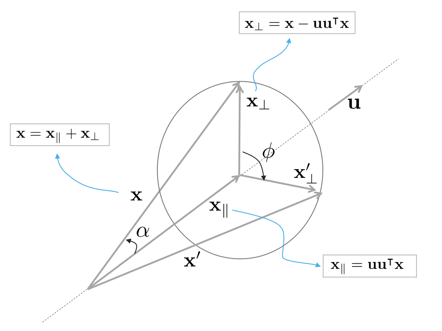
위 그림은 오른손법칙을 사용하여 3차원 공간 상의 임의의 벡터 $\mathbf{x}$를 $\mathbf{u}$축을 중심으로 $\varphi$만큼 회전시키는 모습을 나타낸다. $\mathbf{x}$를 $\mathbf{u}$축에 평행인 벡터 ${\mathbf{x}}_{\parallel }$와 직교하는 벡터 ${\mathbf{x}}_{\perp }$로 분해할 수 있다.
$$\begin{array}{}\text{(56)}& \mathbf{x}={\mathbf{x}}_{\parallel }+{\mathbf{x}}_{\perp }.\end{array}$$

두 벡터는 다음과 같이 계산할 수 있다. 이 때, $\alpha$ 는 $\mathbf{x}$와 $\mathbf{u}$축 사이의 각도를 의미한다.
$$\begin{array}{}\text{(57)}& \begin{array}{rl}& {\mathbf{x}}_{\parallel }=\mathbf{u}(\Vert \mathbf{x}\Vert \cos \alpha )=\mathbf{u}{\mathbf{u}}^{⊺}\mathbf{x}\\ & {\mathbf{x}}_{\perp }=\mathbf{x}-{\mathbf{x}}_{\parallel }=\mathbf{x}-\mathbf{u}{\mathbf{u}}^{⊺}\mathbf{x}.\end{array}\end{array}$$

회전이 수행되는 동안 $\mathbf{u}$축에 평행한 ${\mathbf{x}}_{\parallel }$은 회전하지 않는다.
$$\begin{array}{}\text{(58)}& {\mathbf{x}}_{\parallel }^{\prime }={\mathbf{x}}_{\parallel }\end{array}$$

그리고 $\mathbf{u}$축에 직교하는 파트들은 $\mathbf{u}$와 수직인 평면 내부에서 회전하게 된다. 따라서 평면 내부에 서로 직교하는 두 basis $\{{\mathbf{e}}_1,{\mathbf{e}}_2\}$가 있다고 했을 때 이는 다음과 같이 나타낼 수 있다.
$$\begin{array}{}\text{(59)}& \begin{array}{rl}& {\mathbf{e}}_1={\mathbf{x}}_{\perp }\\ & {\mathbf{e}}_2=\mathbf{u}\times {\mathbf{x}}_{\perp }=\mathbf{u}\times \mathbf{x}\end{array}\end{array}$$

두 basis는 $\Vert {\mathbf{e}}_1\Vert =\Vert {\mathbf{e}}_2\Vert$를 만족한다. 따라서 ${\mathbf{x}}_{\perp }={\mathbf{e}}_1\cdot 1+{\mathbf{e}}_2\cdot 0$과 같이 쓸 수 있고 $\varphi$만큼 회전한 직교벡터에 대해서는 다음과 같이 나타낼 수 있다.
$$\begin{array}{}\text{(60)}& {\mathbf{x}}_{\perp }^{\prime }={\mathbf{e}}_1\cos \varphi +{\mathbf{e}}_2\sin \varphi \end{array}$$

이는 다음과 같이 전개해서 나타낼 수 있다.
$$\begin{array}{}\text{(61)}& {\mathbf{x}}_{\perp }^{\prime }={\mathbf{x}}_{\perp }\cos \varphi +(\mathbf{u}\times \mathbf{x})\sin \varphi \end{array}$$

따라서 최종적으로 회전한 벡터 ${\mathbf{x}}^{\prime }$는 다음과 같이 쓸 수 있다.
$$\begin{array}{}\text{(62)}& \boxed{{\displaystyle {\mathbf{x}}^{\prime }={\mathbf{x}}_{\parallel }^{\prime }+{\mathbf{x}}_{\perp }^{\prime }={\mathbf{x}}_{\parallel }+{\mathbf{x}}_{\perp }\cos \varphi +(\mathbf{u}\times \mathbf{x})\sin \varphi }}\end{array}$$

2.2 The rotation group SO(3)

3차원 공간에서 SO(3) 군은 원점을 중심으로 회전하는 연산에 대한 군을 말한다. 회전은 벡터의 길이와 상대벡터의 방향을 보존하는 선형 변환 연산이다. 이는 로보틱스에서 강체(rigid body)의 움직임 중 회전을 표현하는데 주로 사용된다. 강체의 움직임이란 물체의 형태가 변화하지 않아서 각도, 상대적인 회전량(relative orientation), 거리 등이 보존되는 움직임을 의미한다.

유클리디언 공간에서 $\mathbf{v}\in {\mathbb{R}}^3$ 벡터에 대해 회전을 수행하는 연산자 $r:{\mathbb{R}}^3\to {\mathbb{R}}^3;\mathbf{v}\mapsto r(\mathbf{v})$가 주어졌을 때 이는 다음과 같은 성질을 만족한다.

• 회전은 벡터의 놈을 보존한다.

$$\begin{array}{}\text{(63)}& \Vert r(\mathbf{v})\Vert =\sqrt{<r(\mathbf{v}),r(\mathbf{v})>}=\sqrt{<\mathbf{v},\mathbf{v}>}\triangleq \Vert \mathbf{v}\Vert ,\mathrm{\forall }\mathbf{v}\in {\mathbb{R}}^3\end{array}$$

• 회전은 두 벡터에 대한 각도를 보존한다.

$$\begin{array}{}\text{(64)}& <r(\mathbf{v}),r(\mathbf{w})>=<\mathbf{v},\mathbf{w}>=\Vert \mathbf{v}\Vert \Vert \mathbf{w}\Vert \cos \alpha ,\mathrm{\forall }\mathbf{v},\mathbf{w}\in {\mathbb{R}}^3\end{array}$$

• 회전은 두 벡터의 상대 회전량(relative orientation)을 보존한다.

$$\begin{array}{}\text{(65)}& \mathbf{u}\times \mathbf{v}=\mathbf{w}\iff r(\mathbf{u})\times r(\mathbf{v})=r(\mathbf{w})\end{array}$$


위 성질을 토대로 SO(3) 군을 다음과 같이 정의할 수 있다.
$$\begin{array}{}\text{(66)}& SO(3):\{r:{\mathbb{R}}^3\to {\mathbb{R}}^3/\mathrm{\forall }\mathbf{v},\mathbf{w}\in {\mathbb{R}}^3,\Vert r(\mathbf{v})\Vert =\Vert \mathbf{v}\Vert ,r(\mathbf{v})\times r(\mathbf{w})=r(\mathbf{v}\times \mathbf{w})\}\end{array}$$

SO(3) 군은 일반적으로 회전행렬(rotation matrix)를 사용하여 표기한다. 하지만 쿼터니안을 사용하여 SO(3)를 표기하는 방법 또한 널리 사용된다. 본 챕터에서는 두 표기법이 동일하다는 것을 증명한다. 두 표기법은 개념적으로나 대수적으로 많은 부분에서 유사하다.

2.2 The rotation group and the rotation matrix

회전연산자 $r$은 선형성을 가진다. 따라서 선형성을 가진 스칼라나 벡터, 행렬로도 $r$을 표현할 수 있다. 그 중 대표적인 것이 회전행렬 $\mathbf{R}\in {\mathbb{R}}^{3\times 3}$을 통해 회전연산자를 표현하는 방법이다.
$$\begin{array}{}\text{(67)}& r(\mathbf{v})=\mathbf{Rv}\end{array}$$

내적 $<\mathbf{a},\mathbf{b}>={\mathbf{a}}^{⊺}\mathbf{b}$ 을 활용하여 ($\text{63}$)에 해당 공식을 적용하면 모든 $\mathbf{v}$에 대해 다음 공식이 적용된다.
$$\begin{array}{}\text{(68)}& (\mathbf{Rv}{)}^{⊺}(\mathbf{Rv})={\mathbf{v}}^{⊺}{\mathbf{R}}^{⊺}\mathbf{Rv}={\mathbf{v}}^{⊺}\mathbf{v}.\end{array}$$

이를 통해 회전행렬의 직교하는 성질을 유도할 수 있다.
$$\begin{array}{}\text{(69)}& \boxed{{\displaystyle {\mathbf{R}}^{⊺}\mathbf{R}=\mathbf{I}={\mathbf{RR}}^{⊺}}}\end{array}$$

회전행렬 $\mathbf{R}=[{\mathbf{r}}_1,{\mathbf{r}}_2,{\mathbf{r}}_3]$와 같이 열행렬 ${\mathbf{r}}_i$로 표기하면 직교행렬의 성질에 의해 다음 공식이 성립한다.
$$\begin{array}{}\text{(70)}& \begin{array}{rl}& <{\mathbf{r}}_i,{\mathbf{r}}_i>={\mathbf{r}}_i^{⊺}{\mathbf{r}}_i=1\\ & <{\mathbf{r}}_i,{\mathbf{r}}_j>={\mathbf{r}}_i^{⊺}{\mathbf{r}}_j=0,\text{if }i\ne j\end{array}\end{array}$$

이에 따라 3차원 공간에서 변환 시 벡터의 놈과 각도를 보존하는 군을 Orthogonal 군이라고 하며 줄여서 O(3)라고 표현한다. Orthogonal 군은 강체의 변환일 때 회전과 비강체의 변환일 때 반사(reflection)로 구성되어 있다. 여기서 군이라는 표현을 사용하는 이유는 두 개의 직교하는 O(3) 행렬을 곱하면 언제나 직교하는 O(3) 행렬이 나오기 때문이다. 즉, 곱셈에 대해 닫혀있다. 이는 역행렬 또한 직교행렬의 성질을 만족하는 것을 의미한다. 따라서 ($\text{69}$)에 의해 회전행렬의 역행렬은 전치행렬과 동일하다.
$$\begin{array}{}\text{(71)}& {\mathbf{R}}^{-1}={\mathbf{R}}^{⊺}\end{array}$$

그리고 강체의 움직임에 한해서 상대적인 회전량을 보존하는 성질 ($\text{65}$)에 의해 다음과 같은 제약조건이 추가된다.
$$\begin{array}{}\text{(72)}& \boxed{{\displaystyle det(\mathbf{R})=1}}\end{array}$$

Orthogonal 군에서 특별히 위와같이 positive unit determinant를 만족하는 군을 Speical Orthonogal 군, 즉 SO(3)군이라고 한다. 군의 성질을 만족해야 하므로 임의의 두 SO(3) 회전행렬의 곱은 항상 SO(3) 회전행렬이 된다.

2.3.1 The exponential map

Exponential map(+Logarithm map)은 3차원 공간의 회전을 조금 더 편하게 쉽게 이해 및 응용할 수 있게 해주는 강력한 수학적 도구이다. 이는 미세한 변화량에 대한 미적분(infinitesimal calculus)과 3차원 회전을 연결시켜주는 고리 역할을 수행한다. 또한, 3차원 회전에 대한 자코비안을 정의하거나, 섭동(perturbation) 모델링을 정의하거나 속도를 정의하고 사용할 수 있도록 해주는 핵심적인 역할을 수행한다. 따라서 3차원 공간에서 회전에 대한 추정 문제를 사용할 때 필수적으로 사용된다.

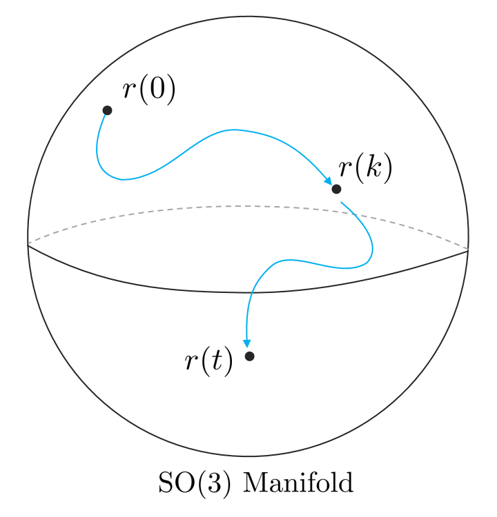
회전은 강체 움직임(rigid motion)의 성질을 만족한다. 이 때, 강체 움직임의 성질이란 처음 $t_0=0$ 순간의 방향 $r(0)$으로부터 $t$ 초 후 현재의 방향 $r(t)$까지 물체가 회전했을 때 SO(3) 군 내에서 연속적인 궤적(continuous trajectory)를 정의할 수 있음을 말한다. 이러한 연속적인 궤적은 시간 $t$에 따라 회전을 미분할 수 있음을 의미한다.

앞서 SO(3)의 제약조건 중 ($\text{69}$)에 대한 시간미분 값을 유도하면 다음과 같다.
$$\begin{array}{}\text{(73)}& \frac{d}{dt}({\mathbf{R}}^{⊺}\mathbf{R})={\dot{\mathbf{R}}}^{⊺}\mathbf{R}+{\mathbf{R}}^{⊺}\dot{\mathbf{R}}=0\end{array}$$

위 식을 정리하면 다음과 같은 공식을 얻을 수 있다.
$$\begin{array}{}\text{(74)}& \begin{array}{r}{\mathbf{R}}^{⊺}\dot{\mathbf{R}}=-({\mathbf{R}}^{⊺}\dot{\mathbf{R}}{)}^{⊺}\end{array}\end{array}$$

이는 ${\mathbf{R}}^{⊺}\dot{\mathbf{R}}$이 반대칭행렬(skew -symmetric matrix)의 성질을 만족하는 것을 의미한다. 이러한 3x3 반대칭행렬의 집합을 so(3)라고 하며 SO(3) 군의 Lie Algebra라고 한다. 3x3 반대칭행렬은 다음과 같은 형태를 갖는다.
$$\begin{array}{}\text{(75)}& \begin{array}{r}{}_{\times }\triangleq \left[\begin{array}{ccc}0& -{\omega }_z& {\omega }_y\\ {\omega }_z& 0& -{\omega }_x\\ -{\omega }_y& {\omega }_x& 0\end{array}\right]\end{array}\end{array}$$

반대칭행렬은 3자유도를 가지며 ($\text{???}$)에서 설명한 것처럼 cross product 연산자로 사용된다. 이는 $\omega \in {\mathbb{R}}^3\leftrightarrow [\omega {]}_{\times }\in so(3)$과 같이 임의의 3차원 벡터는 so(3)와 일대일 매핑 관계에 있다는 것을 알 수 있다.
$$\begin{array}{}\text{(76)}& \begin{array}{r}{\mathbf{R}}^{⊺}\dot{\mathbf{R}}=[\omega {]}_{\times }\end{array}\end{array}$$

위 식은 다음과 같이 일반미분방정식(ordinary differential equation, ODE) 형태를 가진다.
$$\begin{array}{}\text{(77)}& \begin{array}{r}\dot{\mathbf{R}}=\mathbf{R}[\omega {]}_{\times }\end{array}\end{array}$$

원점 부근에서 $\mathbf{R}=I$라고 하면 $\dot{\mathbf{R}}=[\omega {]}_{\times }$의 식이 유도된다. 따라서 so(3)는 원점 근처에서 $r(t)$의 시간에 대한 미분 공간으로 해석할 수 있다. 이는 SO(3) 군에 대한 접평면(tangent space)를 의미한다. 또는 velocity space이라고도 불린다. 따라서, $\omega$는 순간적인 각속도를 의미한다.

만약 각속도 $\omega$가 일정한 경우, 미분방정식은 다음과 같이 나타낼 수 있다.
$$\begin{array}{}\text{(78)}& \begin{array}{r}\mathbf{R}(t)=\mathbf{R}(0)e^{[\omega {]}_{\times }t}={\mathbf{R}}_0{e}^{[\omega t{]}_{\times }}\end{array}\end{array}$$

exponential $e^{[x{]}_{\times }}$는 테일러 급수로 전개하여 나타낼 수 있다. ${\mathbf{R}}_0,\mathbf{R}(t)$는 회전행렬을 의미하므로 $e^{[\omega t{]}_{\times }}=\mathbf{R}(0{)}^{⊺}\mathbf{R}(t)$와 같이 나타낼 수 있다. 임의의 벡터 $\varphi \triangleq \omega \mathrm{\Delta }t$를 시간 $\mathrm{\Delta }t$에 대한 회전벡터로 정의하면 다음 공식을 얻을 수 있다.
$$\begin{array}{}\text{(79)}& \begin{array}{r}\mathbf{R}=e^{[\varphi {]}_{\times }}\end{array}\end{array}$$

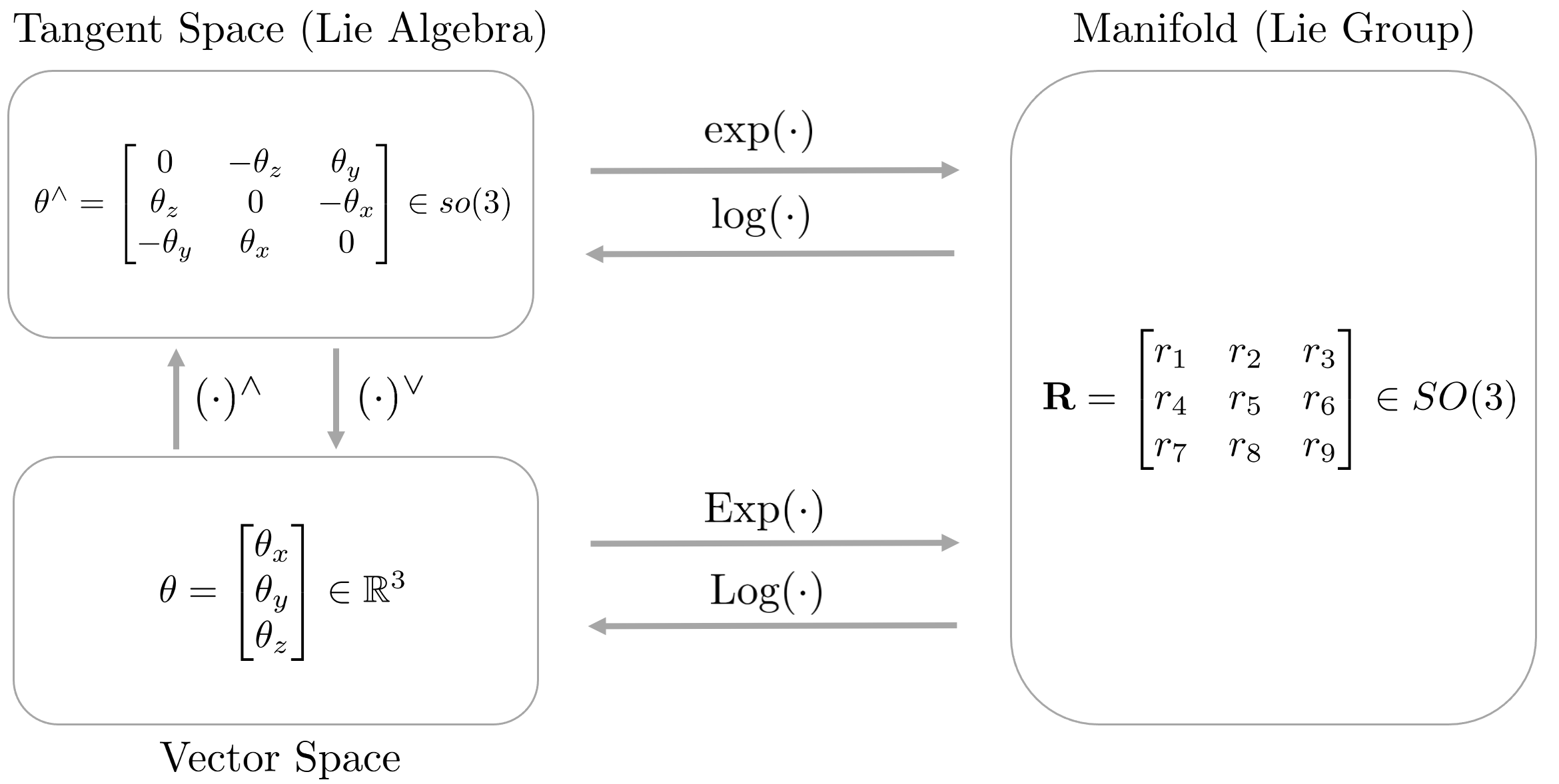
이는 $[\varphi {]}_{\times }$를 exponential map을 통해 회전행렬로 변환이 가능함을 의미한다. 즉, so(3)에서 SO(3) 군으로 변환을 의미한다.
$$\begin{array}{}\text{(80)}& \begin{array}{r}\exp :so(3)\to SO(3);[\varphi {]}_{\times }\mapsto \exp ([\varphi {]}_{\times })=e^{[\varphi {]}_{\times }}\end{array}\end{array}$$

2.3.2 The capitalized exponential map

앞서 소개한 exponential map은 종종 표기법에서 혼란을 일으킨다. 이는 주로 $\varphi \in {\mathbb{R}}^{3]}$와 $[\varphi {]}_{\times }\in so(3)$을 혼용하면서 발생한다. 이러한 표기의 혼란을 막기 위해 ${\mathbb{R}}^3\to SO(3)$로 변환하는 연산은 대문자 $\text{Exp}$ 연산이라고 정의한다.
$$\begin{array}{}\text{(81)}& \begin{array}{r}\text{Exp}:{\mathbb{R}}^3\to SO(3);\varphi \mapsto \text{Exp}(\varphi )=e^{[\varphi {]}_{\times }}\end{array}\end{array}$$

두 연산자 exp, Exp 사이에는 다음과 같은 관계가 성립한다.
$$\begin{array}{}\text{(82)}& \begin{array}{r}\text{Exp}(\varphi )\triangleq \exp ([\varphi {]}_{\times })\end{array}\end{array}$$


다음 섹션에서는 벡터 $\varphi$가 회전벡터 또는 angle-axis 벡터로 불리는 것에 대해 설명한다. 따라서 임의의 각도 $\theta$와 $\mathbf{u}$축에 대해 $\varphi =\omega \mathrm{\Delta }t=\theta \mathbf{u}$와 같이 나타낼 수 있다.

2.3.3 Rotation matrix and rotation vector: the Rodrigues rotation formula

회전행렬 $\mathbf{R}$은 회전벡터 $\varphi =\theta \mathbf{u}$에 exponential map을 적용함으로써 정의된다. ($\text{79}$)에 $\varphi =\theta \mathbf{u}$를 활용하여 테일러 전개해보면 다음과 같다.
$$\begin{array}{}\text{(83)}& \begin{array}{r}\mathbf{R}=e^{\theta [\mathbf{u}{]}_{\times }}=\mathbf{I}+\theta [\mathbf{u}{]}_{\times }+\frac{1}{2}{\theta }^2[\mathbf{u}{]}_{\times }^2+\frac{1}{3!}{\theta }^3[\mathbf{u}{]}_{\times }^3+\frac{1}{4!}{\theta }^4[\mathbf{u}{]}_{\times }^4+\cdots \end{array}\end{array}$$

$\mathbf{u}$는 단위벡터이므로 반대칭행렬 $[\mathbf{u}{]}_{\times }$는 다음을 만족한다.
$$\begin{array}{}\text{(84)}& \begin{array}{rl}& [\mathbf{u}{]}_{\times }^2={\mathbf{uu}}^{⊺}-\mathbf{I}\\ & [\mathbf{u}{]}_{\times }^3=-[\mathbf{u}{]}_{\times }\end{array}\end{array}$$

따라서 모든 $[\mathbf{u}{]}_{\times }$의 지수승은 $[\mathbf{u}{]}_{\times }$와 $[\mathbf{u}{]}_{\times }^2$로 표현이 가능하다.
$$\begin{array}{}\text{(85)}& \begin{array}{r}{}_{\times }^4=-[\mathbf{u}{]}_{\times }^2,[\mathbf{u}{]}_{\times }^5=[\mathbf{u}{]}_{\times },[\mathbf{u}{]}_{\times }^6=[\mathbf{u}{]}_{\times }^2,[\mathbf{u}{]}_{\times }^7=-[\mathbf{u}{]}_{\times },\cdots \end{array}\end{array}$$

따라서 $[\mathbf{u}{]}_{\times }$와 $[\mathbf{u}{]}_{\times }^2$로 테일러 전개를 묶은 후 $\sin \theta$, $\cos \theta$ 공식을 적용하면 회전벡터로부터 회전행렬을 구하는 공식이 나오는데 이를 특별히 Rodrigues rotation formula라고 한다.
$$\begin{array}{}\text{(86)}& \begin{array}{r}\mathbf{R}=\mathbf{I}+\sin \theta [\mathbf{u}{]}_{\times }+(1-\cos \theta )[\mathbf{u}{]}_{\times }^2\end{array}\end{array}$$

이는 $\mathbf{R}\{\theta \}\triangleq \text{Exp}(\theta )$와 같이 나타낼 수 있다. 위 공식은 다양한 변형 공식이 존재하는데 대표적으로 ($\text{84}$)를 활용하여 다음과 같이 나타낼 수 있다.
$$\begin{array}{}\text{(87)}& \begin{array}{r}\mathbf{R}=\mathbf{I}\cos \theta +[\mathbf{u}{]}_{\times }\sin \theta +{\mathbf{uu}}^{⊺}(1-\cos \theta )\end{array}\end{array}$$

2.3.4 The logarithm maps

exponential map의 역연산으로 logarithm map을 정의할 수 있다.
$$\begin{array}{}\text{(88)}& \begin{array}{r}\log :SO(3)\to so(3);\mathbf{R}\mapsto \log (\mathbf{R})=[\mathbf{u}\theta {]}_{\times }\end{array}\end{array}$$

이 때,
$$\begin{array}{}\text{(89)}& \begin{array}{rl}& \theta =\arccos (\frac{\text{trace}(\mathbf{R})-1}{2})\\ & \mathbf{u}=\frac{(\mathbf{R}-{\mathbf{R}}^{⊺}{)}^{\vee }}{2\sin \theta }\end{array}\end{array}$$

와 같으며 $(\cdot {)}^{\vee }$ 연산은 $[\cdot {]}_{\times }$ 연산의 역연산을 의미히나다. 즉, $([\mathbf{v}{]}_{\times }{)}^{\vee }=\mathbf{v}$이고 $[{\mathbf{V}}^{\vee }{]}_{\times }=\mathbf{V}$이다. exponential map과 동일하게 대문자 연산 Log를 정의할 수 있다. 이는 회전행렬로부터 회전벡터를 구하는 연산이다.
$$\begin{array}{}\text{(90)}& \begin{array}{r}\text{Log}:SO(3)\to {\mathbb{R}}^3;\mathbf{R}\mapsto \text{Log}(\mathbf{R})=\mathbf{u}\theta \end{array}\end{array}$$

소문자 연산자와 대문자 연산자 사이에는 다음과 같은 성질을 만족한다.
$$\begin{array}{}\text{(91)}& \begin{array}{r}\text{Log}(\mathbf{R})\triangleq (\log (\mathbf{R}){)}^{\vee }\end{array}\end{array}$$

지금까지 설명한 대소문자 exponential, logarithm map을 그림으로 표현하면 다음과 같다.

2.3.5 The rotation action

3차원 공간에서 임의의 벡터 $\mathbf{x}$를 $\mathbf{u}$축을 중심으로 각도 $\theta$만큼 회전시키기 위해서는 다음과 같은 선형연산이 적용된다.
$$\begin{array}{}\text{(92)}& \begin{array}{r}{\mathbf{x}}^{\prime }=\mathbf{Rx}\end{array}\end{array}$$

이 때, $\mathbf{R}=\text{Exp}(\mathbf{u}\theta )$이다. 이를 Rodrigues formula ($\text{86}$)을 사용하여 표현하면 다음과 같다.
$$\begin{array}{}\text{(93)}& \begin{array}{rl}{\mathbf{x}}^{\prime }& =\mathbf{Rx}\\ & =(\mathbf{I}+\sin \theta [\mathbf{u}{]}_{\times }+(1-\cos \theta )[\mathbf{u}{]}_{\times }^2)\mathbf{x}\\ & =\mathbf{x}+\sin \theta [\mathbf{u}{]}_{\times }\mathbf{x}+(1-\cos \theta )[\mathbf{u}{]}_{\times }^2\mathbf{x}\\ & =\mathbf{x}+\sin \theta (\mathbf{u}\times \mathbf{x})+(1-\cos \theta )({\mathbf{uu}}^{⊺}-\mathbf{I})\mathbf{x}\\ & ={\mathbf{x}}_{\parallel }+{\mathbf{x}}_{\perp }+\sin \theta (\mathbf{u}\times \mathbf{x})-(1-\cos \theta ){\mathbf{x}}_{\perp }\\ & ={\mathbf{x}}_{\parallel }+(\mathbf{u}\times \mathbf{x})\sin \theta +{\mathbf{x}}_{\perp }\cos \theta \end{array}\end{array}$$

이는 정확히 벡터의 회전 공식 ($\text{62}$)과 동일하다.

2.4 The rotation group and the quaternion

본 섹션에서는 SO(3)의 표기법으로 쿼터니언을 사용하는 방법에 대해 설명한다. 또한, 쿼터니언과 회전행렬이 어떠한 연관성이 있는지 설명한다. 쿼터니언이 벡터를 회전하는 연산은 다음과 같이 나타낼 수 있다.
$$\begin{array}{}\text{(94)}& \begin{array}{r}r(\mathbf{v})=\mathbf{q}\otimes \mathbf{v}\otimes {\mathbf{q}}^{\ast }\end{array}\end{array}$$

또한, 이를 통해 제약조건 ($\text{30}$)를 활용하여 ($\text{63}$)를 다시 표기하면 다음과 같다.
$$\begin{array}{}\text{(95)}& \begin{array}{r}\Vert \mathbf{q}\otimes \mathbf{v}\otimes {\mathbf{q}}^{\ast }\Vert ={\Vert \mathbf{q}\Vert }^2\Vert \mathbf{v}\Vert =\Vert \mathbf{v}\Vert \end{array}\end{array}$$

이를 통해 $\Vert \mathbf{q}\Vert =1$ 조건을 유도할 수 있다. 즉, 단위 쿼터니언(unit quaternion)만이 물체의 3차원 회전에 대한 연산을 수행할 수 있음을 의미한다. 이를 통해 다음 공식이 성립한다
$$\begin{array}{}\text{(96)}& \begin{array}{r}\boxed{{\displaystyle {\mathbf{q}}^{\ast }\otimes \mathbf{q}=1=\mathbf{q}\otimes {\mathbf{q}}^{\ast }}}\end{array}\end{array}$$

이는 회전행렬의 직교성질인 ${\mathbf{R}}^{⊺}\mathbf{R}=\mathbf{I}={\mathbf{RR}}^{⊺}$ ($\text{69}$)와 유사하다. 또한 아래와 같은 전개를 통해 ($\text{65}$)이 성립함을 보일 수 있다.
$$\begin{array}{}\text{(97)}& \begin{array}{rlrl}& r(\mathbf{v})\times r(\mathbf{w})& & =(\mathbf{q}\otimes \mathbf{v}\otimes {\mathbf{q}}^{\ast })\times (\mathbf{q}\otimes \mathbf{w}\otimes {\mathbf{q}}^{\ast })\\ & (\text{36})& & =\frac{1}{2}((\mathbf{q}\otimes \mathbf{v}\otimes {\mathbf{q}}^{\ast })\otimes (\mathbf{q}\otimes \mathbf{w}\otimes {\mathbf{q}}^{\ast })-(\mathbf{q}\otimes \mathbf{w}\otimes {\mathbf{q}}^{\ast })\otimes (\mathbf{q}\otimes \mathbf{v}\otimes {\mathbf{q}}^{\ast }))\\ & & & =\frac{1}{2}(\mathbf{q}\otimes \mathbf{v}\otimes \mathbf{w}\otimes {\mathbf{q}}^{\ast }-\mathbf{q}\otimes \mathbf{w}\otimes \mathbf{v}\otimes {\mathbf{q}}^{\ast })\\ & & & =\frac{1}{2}(\mathbf{q}\otimes (\mathbf{v}\otimes \mathbf{w}-\mathbf{w}\otimes \mathbf{v})\otimes {\mathbf{q}}^{\ast })\\ & (\text{36})& & =\mathbf{q}\otimes (\mathbf{v}\times \mathbf{w})\otimes {\mathbf{q}}^{\ast }\\ & & & =r(\mathbf{v}\times \mathbf{w})\end{array}\end{array}$$

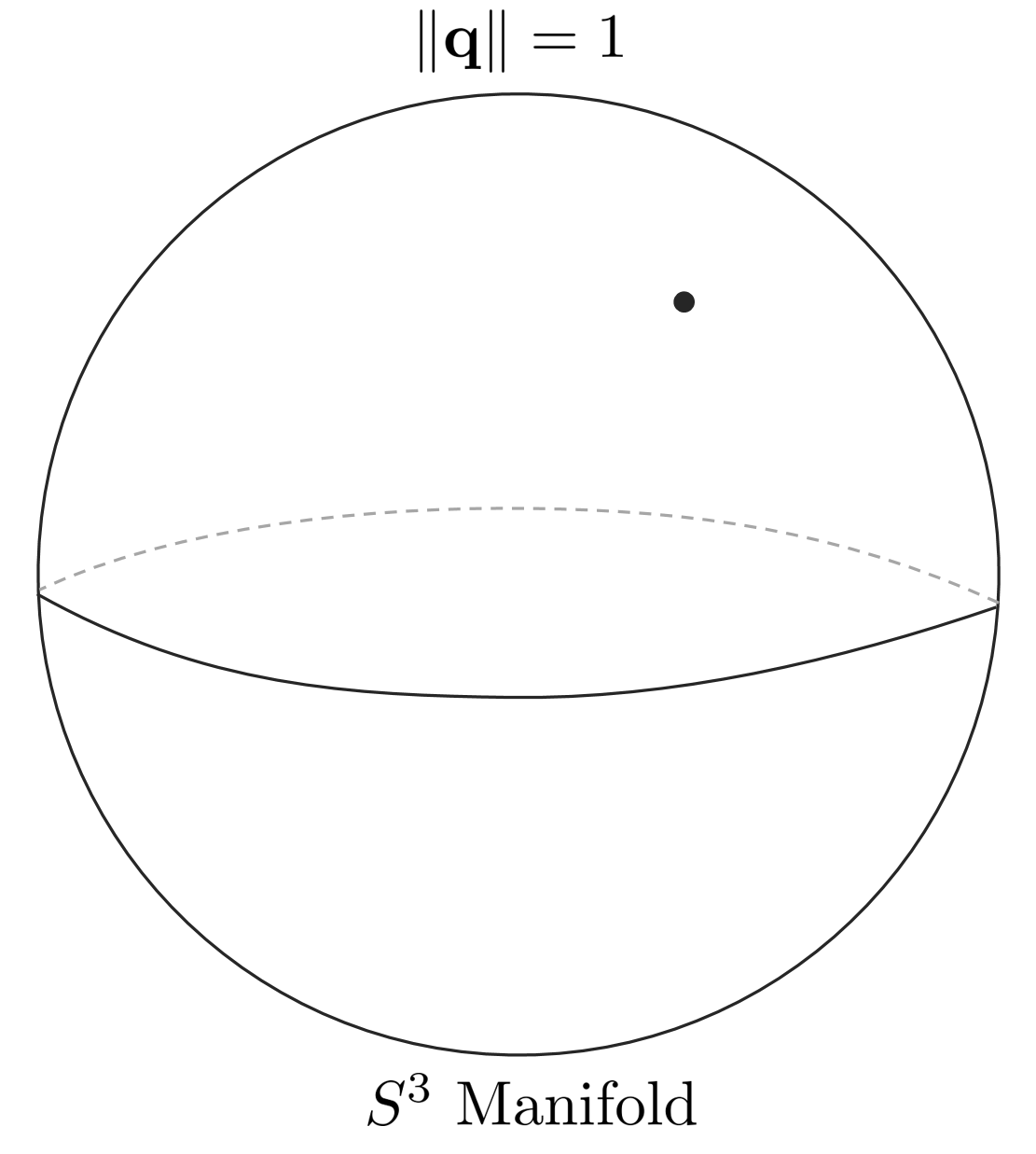
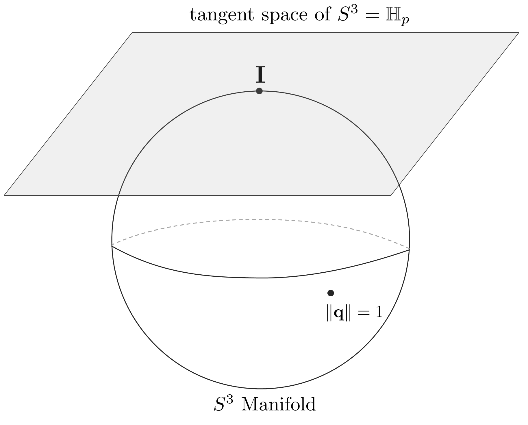
위 전개를 통해 단위 쿼터니언은 곱셈 연산에 대해 닫힌 연산을 수행하는 군을 형성하는 것을 알 수 있다. 단위 쿼터니언 군의 manifold는 기하학적으로 ${\mathbb{R}}^4$차원의 단위 구(unit sphere)를 형성한다. 4차원 구는 일반적으로 표현할 수 없으므로 이를 단순화하여 3차원 구를 통해 manifold를 설명한다. 이러한 단위 쿼터니언의 군을 ${\mathcal{S}}^3$라고 부른다.

2.4.1 The exponential map

임의의 단위 쿼터니언이 $\mathbf{q}\in S^3$가 주어졌을 때 이는 직교조건 ${\mathbf{q}}^{\ast }\otimes \mathbf{q}=1$을 만족한다. 따라서 회전행렬과 마찬가지로 직교조건에 대해 미분을 취하면 다음과 같다.
$$\begin{array}{}\text{(98)}& \frac{d({\mathbf{q}}^{\ast }\otimes \mathbf{q})}{dt}={\dot{\mathbf{q}}}^{\ast }\otimes \mathbf{q}+{\mathbf{q}}^{\ast }\otimes \dot{\mathbf{q}}=0\end{array}$$

이를 전개하면 다음과 같다.
$$\begin{array}{}\text{(99)}& {\mathbf{q}}^{\ast }\otimes \dot{\mathbf{q}}=-({\dot{\mathbf{q}}}^{\ast }\otimes \mathbf{q})=-({\mathbf{q}}^{\ast }\otimes \dot{\mathbf{q}}{)}^{\ast }\end{array}$$

이는 곧 ${\mathbf{q}}^{\ast }\otimes \dot{\mathbf{q}}$이 순수 쿼터니언임(pure quaternion)을 의미한다. 순수 쿼터니언은 실수부가 0이므로 켤레복소수를 취하면 음수인 자기 자신이 된다. 순수 쿼터니언을 $\mathrm{\Omega }\in \mathbb{H}$라고 하면 다음과 같이 나타낼 수 있다.
$$\begin{array}{}\text{(100)}& {\mathbf{q}}^{\ast }\otimes \dot{\mathbf{q}}=\mathrm{\Omega }=\left[\begin{array}{c}0\\ \mathrm{\Omega }\end{array}\right]\in {\mathbb{H}}_p\end{array}$$

이를 정리하면 다음과 같다.
$$\begin{array}{}\text{(101)}& \dot{\mathbf{q}}=\mathbf{q}\otimes \mathrm{\Omega }\end{array}$$

원점 부근에서 $\mathbf{q}=1$이 되고 위 식은 $\dot{\mathbf{q}}=\mathrm{\Omega }\in {\mathbb{H}}_p$와 같이 나타낼 수 있다. 따라서 순수 쿼터니언 공간 ${\mathbb{H}}_p$는 접평면(tangent space)을 의미하며 $S^3$ 군의 Lie Algebra라고 불린다.

단위 쿼터니언의 경우 회전행렬과 달리 접평면이 velocity space를 의미하지 않고 half-velocity space를 의미한다. 이에 대해서는 뒷 섹션에서 자세히 설명한다. 만약 $\mathrm{\Omega }$가 일정한 경우 미분방정식은 다음과 같이 나타낼 수 있다.
$$\begin{array}{}\text{(102)}& \mathbf{q}(t)=\mathbf{q}(0)\otimes e^{\mathrm{\Omega }t}\end{array}$$

위 식에서 $\mathbf{q}(t)$와 ${\mathbf{q}}_0$가 모두 단위 쿼터니언이므로 $e^{\mathrm{\Omega }t}$ 또한 단위 쿼터니언이 된다. 이는 ($\text{45}$)에서 한 번 유도한 적이 있다. $\mathbf{V}\triangleq \mathrm{\Omega }\mathrm{\Delta }t$와 같이 정의하면
$$\begin{array}{}\text{(103)}& \boxed{{\displaystyle \mathbf{q}=e^{\mathbf{V}}}}\end{array}$$

와 같이 나타낼 수 있다. 이는 회전행렬과 마찬가지로 순수 쿼터니언(pure quaterinon)에 exponential map을 취하면 단위 쿼터니언(unit quaternion)을 만들 수 있음을 의미한다.
$$\begin{array}{}\text{(104)}& \exp :{\mathbb{H}}_p\to S^3;\mathbf{V}\mapsto \exp (\mathbf{V})=e^{\mathbf{V}}\end{array}$$

2.4.2 The capitalized exponential map

exponential map에 사용되는 순수 쿼터니언 $\mathbf{V}$은 일반적으로 $\mathbf{V}=\theta \mathbf{u}=\varphi \mathbf{u}/2$와 같이 $\mathbf{u}$축을 중심으로 회전하고자 하는 각도 $\varphi$의 절반의 각도 $\theta =\varphi /2$를 사용한다. 이에 대해 직관적으로 이해해보면 다음과 같다. 임의의 벡터 $\mathbf{x}$가 쿼터니언에 의해 회전하기 위해서는 ${\mathbf{x}}^{\prime }=\mathbf{q}\otimes \mathbf{x}\otimes {\mathbf{q}}^{\ast }$과 같이 두 번에 걸쳐서 쿼터니언이 곱해지기 때문에 $\mathbf{V}$에 절반의 각도를 사용하는 것으로 이해할 수 있다.

쿼터니언과 angle-axis 표현법 $\mathbf{v}=\varphi \mathbf{u}\in {\mathbb{R}}^3$ 사이의 직접적인 관계를 표현하기 위해 angle-axis의 절반의 각도를 사용하는 순수 쿼터니언으로 변환하는 대문자 exponential map에 대해 정의할 수 있다.
$$\begin{array}{}\text{(105)}& \text{Exp}:{\mathbb{R}}^3\to S^3;\mathbf{v}\mapsto \text{Exp}(\mathbf{v})=e^{\mathbf{v}/2}\end{array}$$

대문자와 소문자 exponential map 사이의 관계는 다음과 같다.
$$\begin{array}{}\text{(106)}& \text{Exp}(\mathbf{v})\triangleq \exp (\mathbf{v}/2)\end{array}$$

임의의 각속도를 $\omega =2\mathrm{\Omega }\in {\mathbb{R}}^3$와 같이 정의하면 ($\text{101}$), ($\text{102}$)은 다음과 같이 다시 나타낼 수 있다.
$$\begin{array}{}\text{(107)}& \begin{array}{rl}& \dot{\mathbf{q}}=\frac{1}{2}\mathbf{q}\otimes \omega \\ & \mathbf{q}=e^{\omega t/2}\end{array}\end{array}$$

2.4.3 Quaternion and rotation vector

임의의 angle-axis 벡터 $\mathbf{v}=\varphi \mathbf{u}$가 주어졌을 때, 이에 대한 exponential map은 오일러 공식의 확장 버전으로 표현할 수 있다.
$$\begin{array}{}\text{(108)}& \boxed{{\displaystyle \mathbf{q}\triangleq \text{Exp}(\mathbf{v})=\text{Exp}(\varphi \mathbf{u})=e^{\varphi \mathbf{u}/2}=\cos \frac{\varphi }{2}+\mathbf{u}\sin \frac{\varphi }{2}=\left[\begin{array}{c}\cos (\varphi /2)\\ \mathbf{u}\sin (\varphi /2)\end{array}\right]}}\end{array}$$

위 식은 주로 angle-axis 표현법에서 쿼터니언으로 변환하는 공식으로 사용되며 $\mathbf{q}=\mathbf{q}\{\mathbf{v}\}\triangleq \text{Exp}(\mathbf{v})$와 같이 표기한다.

2.4.4 The logarithmic maps

단위 쿼터니언 또한 회전행렬과 마찬가지로 exponential map에 대한 역연산인 logarithmic map이 존재한다.
$$\begin{array}{}\text{(109)}& \log :S^3\to {\mathbb{H}}_p;\mathbf{q}\mapsto \log (\mathbf{q})=\mathbf{u}\theta \end{array}$$

또한 대문자 logratihmic map 역시 존재한다. 이는 임의의 쿼터니언을 3차원 벡터로 변환하는 연산이다.
$$\begin{array}{}\text{(110)}& \text{Log}:S^3\to {\mathbb{R}}^3;\mathbf{q}\mapsto \text{Log}(\mathbf{q})=\mathbf{u}\varphi \end{array}$$

두 연산 사이에는 다음과 같은 관계가 성립한다.
$$\begin{array}{}\text{(111)}& \text{Log}(\mathbf{q})\triangleq 2\log (\mathbf{q})\end{array}$$

$\varphi$와 $\mathbf{u}$는 다음과 같이 구할 수 있다.
$$\begin{array}{}\text{(112)}& \begin{array}{rl}& \varphi =2\arctan (\Vert {\mathbf{q}}_v\Vert ,q_w)\\ & \mathbf{u}={\mathbf{q}}_v/\Vert {\mathbf{q}}_v\Vert \end{array}\end{array}$$

매우 작은 움직임을 표현하는 쿼터니언에 대해서는 위 식과 같이 $\mathbf{u}$를 구할 수 없다. 이럴 경우에는 테일러 급수를 사용하여 고차항을 버리고 근사된 값을 사용한다.
$$\begin{array}{}\text{(113)}& \text{Log}(\mathbf{q})=\theta \mathbf{u}\simeq 2\frac{{\mathbf{q}}_v}{q_w}(1-\frac{{\Vert {\mathbf{q}}_v\Vert }^2}{3q_w^2})\end{array}$$

2.4.5 The rotation action

앞서 설명한 내용과 같이 3차원 공간에서 임의의 벡터 $\mathbf{x}$를 $\mathbf{u}$축을 중심으로 $\varphi$만큼 회전하고 싶으면 다음과 같이 2번의 쿼터니언 곱을 통해 회전을 표현할 수 있다.
$$\begin{array}{}\text{(114)}& {\mathbf{x}}^{\prime }=\mathbf{q}\otimes \mathbf{x}\otimes {\mathbf{q}}^{\ast }\end{array}$$

이 때, $\mathbf{q}=\text{Exp}(\mathbf{u}\varphi )$를 의미하며 임의의 벡터 $\mathbf{x}$ 또한 다음과 같은 쿼터니언 형태로 변형된다.
$$\begin{array}{}\text{(115)}& \mathbf{x}=xi+yj+zk=\left[\begin{array}{c}0\\ \mathbf{x}\end{array}\right]\in {\mathbb{H}}_p\end{array}$$

2번의 쿼터니언 곱이 벡터의 회전을 수행하는 것을 증명하기 위해서 ($\text{13}$), ($\text{107}$)를 사용하여 위 공식을 다음과 같이 나타낼 수 있다.
$$\begin{array}{}\text{(116)}& \begin{array}{rl}{\mathbf{x}}^{\prime }& =\mathbf{q}\otimes \mathbf{x}\otimes {\mathbf{q}}^{\ast }\\ & =(\cos \frac{\varphi }{2}+\mathbf{u}\sin \frac{\varphi }{2})\otimes (0+\mathbf{x})\otimes (\cos \frac{\varphi }{2}-\mathbf{u}\sin \frac{\varphi }{2})\\ & =\mathbf{x}{\cos }^2\frac{\varphi }{2}+(\mathbf{u}\otimes \mathbf{x}-\mathbf{x}\otimes \mathbf{u})\sin \frac{\varphi }{2}\cos \frac{\varphi }{2}-\mathbf{u}\otimes \mathbf{x}\otimes \mathbf{u}{\sin }^2\frac{\varphi }{2}\\ & =\mathbf{x}{\cos }^2\frac{\varphi }{2}+2(\mathbf{u}\times \mathbf{x})\sin \frac{\varphi }{2}\cos \frac{\varphi }{2}-(\mathbf{x}({\mathbf{u}}^{⊺}\mathbf{u})-2\mathbf{u}({\mathbf{u}}^{⊺}\mathbf{x})){\sin }^2\frac{\varphi }{2}\\ & =\mathbf{x}({\cos }^2\frac{\varphi }{2}-{\sin }^2\frac{\varphi }{2})+(\mathbf{u}\times \mathbf{x})(2\sin \frac{\varphi }{2}\cos \frac{\varphi }{2})+\mathbf{u}({\mathbf{u}}^{⊺}\mathbf{x})(2{\sin }^2\frac{\varphi }{2})\\ & =\mathbf{x}\cos \varphi +(\mathbf{u}\times \mathbf{x})\sin \varphi +\mathbf{u}({\mathbf{u}}^{⊺}\mathbf{x})(1-\cos \varphi )\\ & =(\mathbf{x}-{\mathbf{uu}}^{⊺}\mathbf{x})\cos \varphi +(\mathbf{u}\times \mathbf{x})\sin \varphi +{\mathbf{uu}}^{⊺}\mathbf{x}\\ & ={\mathbf{x}}_{\perp }\cos \varphi +(\mathbf{u}\times \mathbf{x})\sin \varphi +{\mathbf{x}}_{\parallel }\end{array}\end{array}$$

위 전개를 통해 쿼터니언 연산이 벡터의 회전 공식과 동일하다는 것을 알 수 있다.

2.4.6 The double cover of the manifold of SO(3)

임의의 단위 쿼터니언 $\mathbf{q}$가 주어졌다고 했을 때, 항등 쿼터니언(identity quaternion) ${\mathbf{q}}_1=[1,0,0,0]$과 $\mathbf{q}$ 사이의 각도 $\theta$는 다음과 같이 표현할 수 있다.
$$\begin{array}{}\text{(117)}& \cos \theta ={\mathbf{q}}_1^{⊺}\mathbf{q}=\mathbf{q}(1)=q_w\end{array}$$

또한, 3차원 물체가 $\mathbf{q}$에 의해 $\varphi$ 각도만큼 회전했을 때 $\mathbf{q}$는 다음과 같다.
$$\begin{array}{}\text{(118)}& \mathbf{q}=\left[\begin{array}{c}{q}_w\\ {\mathbf{q}}_v\end{array}\right]=\left[\begin{array}{c}\cos \varphi /2\\ \mathbf{u}\sin \varphi /2\end{array}\right]\end{array}$$

위 두 식을 종합해보면 $q_w=\cos \theta =\cos \varphi /2$인 것을 알 수 있다. 즉, 단위 쿼터니언 공간 $S^3$에서 움직이는 각도 $\theta$는 실제 물체가 움직이는 각도의 절반 $\varphi /2$ 인 것을 알 수 있다.
$$\begin{array}{}\text{(119)}& \theta =\varphi /2\end{array}$$

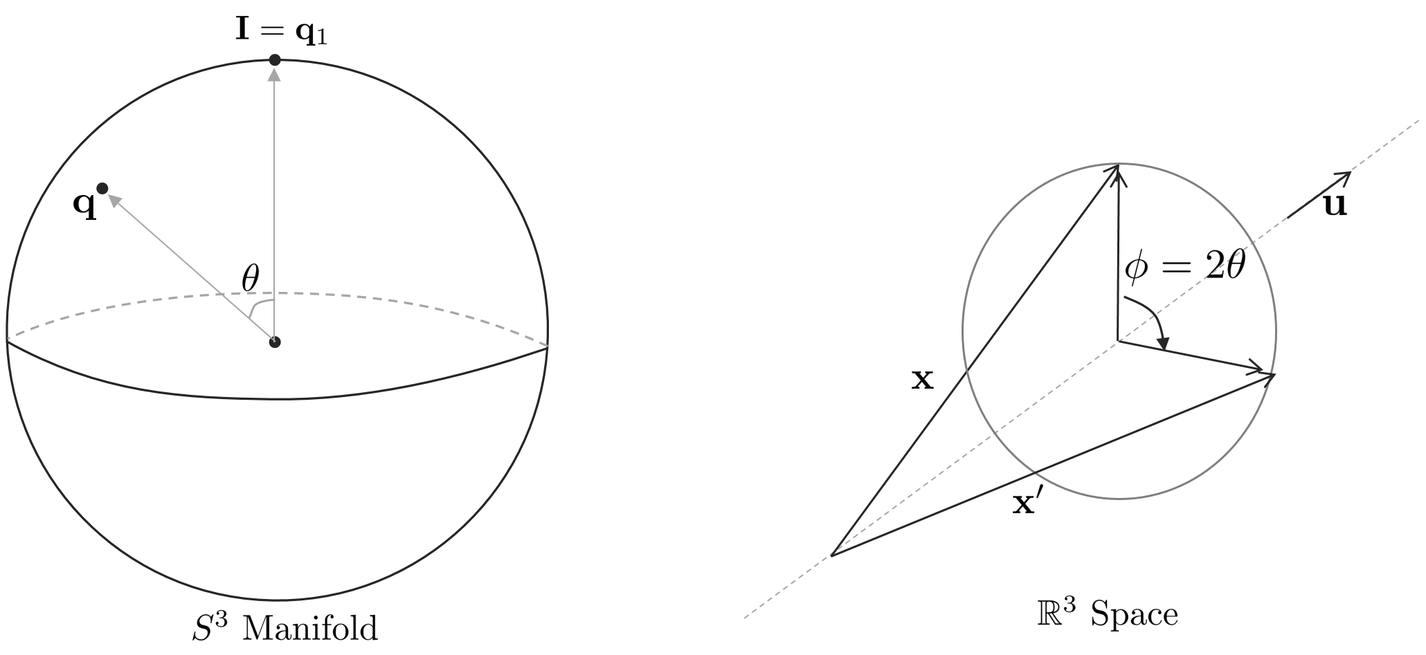
만약 $\theta =\pi /2$인 경우 실제 월드 상의 물체는 $\varphi =\pi$만큼 회전한다. 그리고 $\theta =\pi$만큼 반바퀴 회전을 하면 실제 월드 상의 물체는 $\varphi =2\pi$만큼 한 바퀴 회전을 한다.

2.5 Rotation matrix and quaternion

임의의 angle-axis 벡터 $\mathbf{v}=\mathbf{u}\varphi$가 주어졌을 때, $\mathbf{q}=\text{Exp}(\mathbf{u}\varphi )$를 통해 단위 쿼터니언을 만들 수 있고 또한 $\mathbf{R}=\text{Exp}(\mathbf{u}\varphi )$를 통해 회전행렬을 만들 수 있다. 그리고 위 두 값을 통해 3차원 공간 상의 임의의 벡터 $\mathbf{x}$를 $\mathbf{u}$축을 중심으로 $\varphi$만큼 회전시킬 수 있다.
$$\begin{array}{}\text{(120)}& \mathrm{\forall }\mathbf{v},\mathbf{x}\in {\mathbb{R}}^3,\mathbf{q}=\text{Exp}(\mathbf{v}),\mathbf{R}=\text{Exp}(\mathbf{v})\end{array}$$

이는 곧 다음 공식이 성립함을 의미한다.
$$\begin{array}{}\text{(121)}& \mathbf{q}\otimes \mathbf{x}\otimes {\mathbf{q}}^{\ast }=\mathbf{Rx}\end{array}$$

위 두 식은 모두 $\mathbf{x}$에 대한 선형변환 식이다. 이를 토대로 회전행렬과 단위 쿼터니언 사이의 변환식을 다음과 같이 유도할 수 있다.
$$\begin{array}{}\text{(122)}& \boxed{{\displaystyle \mathbf{R}=\left[\begin{array}{ccc}{q}_w^2+q_x^2-q_y^2-q_z^2& 2(q_x{q}_y-q_w{q}_z)& 2(q_x{q}_z+q_w{q}_y)\\ 2(q_x{q}_y+q_w{q}_z)& q_w^2-q_x^2+q_y^2-q_z^2& 2(q_y{q}_z-q_w{q}_x)\\ 2(q_x{q}_z-q_w{q}_y)& 2(q_y{q}_z+q_w{q}_z)& q_w^2-q_x^2-q_y^2+q_z^2\end{array}\right]}}\end{array}$$

위 변환식은 $\mathbf{R}=\mathbf{R}\{\mathbf{q}\}$와 같이 나타낸다. 또한, ($\text{???}$)를 참고해서 쿼터니언을 행렬곱 형태로 만들면 다음과 같이 다시 쓸 수 있다.
$$\begin{array}{}\text{(123)}& \mathbf{q}\otimes \mathbf{x}\otimes {\mathbf{q}}^{\ast }=[{\mathbf{q}}^{\ast }{]}_R[\mathbf{q}{]}_L\left[\begin{array}{c}0\\ \mathbf{x}\end{array}\right]=\left[\begin{array}{c}0\\ \mathbf{Rx}\end{array}\right]\end{array}$$

이를 통해 다음과 같이 다른 변환 공식을 유도할 수 있다.
$$\begin{array}{}\text{(124)}& \boxed{{\displaystyle \mathbf{R}=(q_w^2-{\mathbf{q}}_v^{⊺}{\mathbf{q}}_v)\mathbf{I}+2{\mathbf{q}}_v{\mathbf{q}}_v^{⊺}+2q_w[{\mathbf{q}}_v{]}_{\times }}}\end{array}$$

회전행렬과 단위 쿼터니언 사이에는 다음과 같은 성질이 만족한다.
$$\begin{array}{}\text{(125)}& \begin{array}{rl}& \mathbf{R}\{[1,0,0,0{]}^{⊺}\}=\mathbf{I}\\ & \mathbf{R}\{\mathbf{-}\mathbf{q}\}=\mathbf{R}\{\mathbf{q}\}\\ & \mathbf{R}\{{\mathbf{q}}^{\ast }\}=\mathbf{R}\{\mathbf{q}{\}}^{⊺}\\ & \mathbf{R}\{{\mathbf{q}}_1\otimes {\mathbf{q}}_2\}=\mathbf{R}\{{\mathbf{q}}_1\}\mathbf{R}\{{\mathbf{q}}_2\}\end{array}\end{array}$$

위 성질들을 토대로 쿼터니언의 지수승은 다음과 같이 변환된다.
$$\begin{array}{}\text{(126)}& \mathbf{R}\{{\mathbf{q}}^t\}=\mathbf{R}\{\mathbf{q}{\}}^t\end{array}$$

이는 스칼라 $t$에 대해 단위 쿼터니언과 회전행렬의 구형 보간법(spherical interpolation)이 서로 연관이 있음을 의미한다.

2.6 Rotation composition

단위 쿼터니언의 합성(composition)은 회전함수의 합성과 유사하다. 즉, 동일한 순서로 곱셈을 수행한다.
$$\begin{array}{}\text{(127)}& {\mathbf{q}}_{AC}={\mathbf{q}}_{AB}\otimes {\mathbf{q}}_{BC}{\mathbf{R}}_{AC}={\mathbf{R}}_{AB}{\mathbf{R}}_{BC}\end{array}$$

이는 결합법칙을 사용하여 다음과 같이 나타낼 수 있다.
$$\begin{array}{}\text{(128)}& \begin{array}{rl}{\mathbf{x}}_A& ={\mathbf{q}}_{AB}\otimes {\mathbf{x}}_B\otimes {\mathbf{q}}_{AB}^{\ast }\\ & ={\mathbf{q}}_{AB}\otimes ({\mathbf{q}}_{BC}\otimes {\mathbf{x}}_c\otimes {\mathbf{q}}_{BC}^{\ast })\otimes {\mathbf{q}}_{AB}^{\ast }\\ & =({\mathbf{q}}_{AB}\otimes {\mathbf{q}}_{BC})\otimes {\mathbf{x}}_c\otimes ({\mathbf{q}}_{BC}^{\ast }\otimes {\mathbf{q}}_{AB}^{\ast })\\ & =({\mathbf{q}}_{AB}\otimes {\mathbf{q}}_{BC})\otimes {\mathbf{x}}_c\otimes ({\mathbf{q}}_{AB}\otimes {\mathbf{q}}_{BC}{)}^{\ast }\\ & ={\mathbf{q}}_{AC}\otimes {\mathbf{x}}_c\otimes {\mathbf{q}}_{AC}^{\ast }\text{for quaternion}\end{array}\end{array}$$

$$\begin{array}{}\text{(129)}& \begin{array}{rl}{\mathbf{x}}_A& ={\mathbf{R}}_{AB}{\mathbf{x}}_B\\ & ={\mathbf{R}}_{AB}({\mathbf{R}}_{BC}{\mathbf{x}}_C)\\ & =({\mathbf{R}}_{AB}{\mathbf{R}}_{BC}){\mathbf{x}}_C\\ & ={\mathbf{R}}_{AC}{\mathbf{x}}_C\text{for rotation matrix}\end{array}\end{array}$$

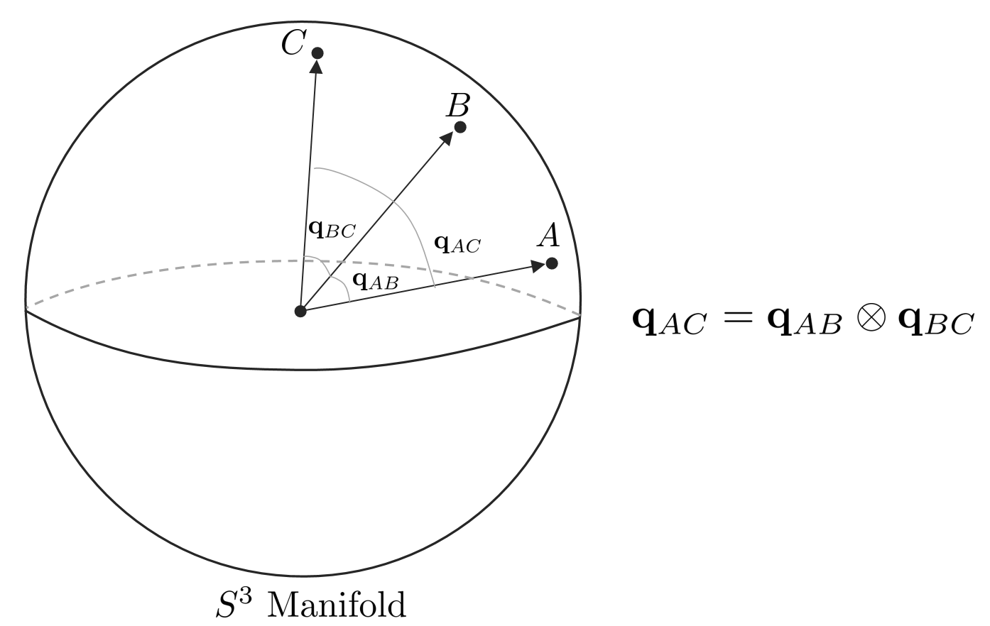
이 때, ${\mathbf{q}}_{ij}$ 또는 ${\mathbf{R}}_{ij}$의 의미는 특정 i 방향(orientation)에서 j 방향으로 변환하는 연산자를 의미한다. 또는 i 좌표계에서 j 좌표계로의 변환으로도 이해할 수 있다.

2.7 Spherical linear interpolation (SLERP)

단위 쿼터니언은 두 방향(orientation) ${\mathbf{q}}_0,{\mathbf{q}}_1$이 주어졌을 때 두 지점을 구의 선형 보간(spherical linear interpolation)하기 상대적으로 쉬운 특징을 가지고 있다. 구의 선형보간은 출발지가 ${\mathbf{q}}_0$ 이고 목적지가 ${\mathbf{q}}_1$일 때, 특정 시간 $t$에서 보간함수 $\mathbf{q}(t),t\in [0,1]$를 구하는 문제가 된다. 보간함수는 초기조건으로 $\mathbf{q}(0)={\mathbf{q}}_0,\mathbf{q}(1)={\mathbf{q}}_1$를 가진다. 보간함수 $\mathbf{q}(t)$를 사용하면 $t\in [0,1]$ 구간에서 물체가 고정된 속도로 자연스럽게 ${\mathbf{q}}_0\to {\mathbf{q}}_1$로 회전할 수있다.

Method 1 첫 번째 방법은 쿼터니언 대수학을 이용하는 것이다. 방향의 변화량 $\mathrm{\Delta }\mathbf{q}$를 사용하여 ${\mathbf{q}}_1={\mathbf{q}}_0\otimes \mathrm{\Delta }{\mathbf{q}}_0$와 같이 표현하는 방법이다.
$$\begin{array}{}\text{(130)}& \mathrm{\Delta }\mathbf{q}={\mathbf{q}}_0^{\ast }\otimes {\mathbf{q}}_1\end{array}$$

위 변화량에 logarithmic map을 사용하여 angle-axis 회전벡터 $\mathrm{\Delta }\mathbf{v}=\mathbf{u}\mathrm{\Delta }\varphi$를 얻을 수 있다.
$$\begin{array}{}\text{(131)}& \mathbf{u}\mathrm{\Delta }\varphi =\text{Log}(\mathrm{\Delta }\mathbf{q})\end{array}$$

최종적으로 $\mathbf{u}$축은 유지한 상태에서 시간 $t\in [0,1]$에 따른 각도의 변화량을 $\delta \varphi =t\mathrm{\Delta }\varphi$라고 하면 $\delta \mathbf{q}=\text{Exp}(\mathbf{u}\delta \varphi )$와 같이 나타낼 수 있다. 이를 다시 위 공식에 대입하면 다음과 같이 보간함수를 구할 수 있다.
$$\begin{array}{}\text{(132)}& \mathbf{q}(t)={\mathbf{q}}_0\otimes \text{Exp}(t\mathbf{u}\mathrm{\Delta }\varphi )\end{array}$$

이를 자세히 풀어쓰면 $\mathbf{q}(t)={\mathbf{q}}_0\otimes \text{Exp}(t\text{Log}({\mathbf{q}}_0^{\ast }\otimes {\mathbf{q}}_1))$가 되고 이를 다시 정리하면 다음과 같다.
$$\begin{array}{}\text{(133)}& \boxed{{\displaystyle \mathbf{q}(t)={\mathbf{q}}_0\otimes ({\mathbf{q}}_0^{\ast }\otimes {\mathbf{q}}_1{)}^t}}\end{array}$$

이는 ($\text{55}$)과 같이 벡터 형태로 나타낼 수 있다.
$$\begin{array}{}\text{(134)}& \mathbf{q}(t)={\mathbf{q}}_0\otimes \left[\begin{array}{c}\cos (t\mathrm{\Delta }\varphi /2)\\ \mathbf{u}\sin (t\mathrm{\Delta }\varphi /2)\end{array}\right]\end{array}$$

Note: 위 식을 회전행렬에 대한 식으로 변경하면 다음과 같다.
$$\begin{array}{}\text{(135)}& \mathbf{R}(t)={\mathbf{R}}_0\text{Exp}(t\text{Log}({\mathbf{R}}_0^{⊺}{\mathbf{R}}_1))={\mathbf{R}}_0({\mathbf{R}}_0^{⊺}{\mathbf{R}}_1{)}^t\end{array}$$

${\mathbf{R}}^t$를 Rodrigues 공식 ($\text{86}$)을 사용하여 다시 표현하면 다음과 같다.
$$\begin{array}{}\text{(136)}& \mathbf{R}(t)={\mathbf{R}}_0(\mathbf{I}+\sin (t\mathrm{\Delta }\varphi )[\mathbf{u}{]}_{\times }+(1-\cos (t\mathrm{\Delta }\varphi ))[\mathbf{u}{]}_{\times })\end{array}$$

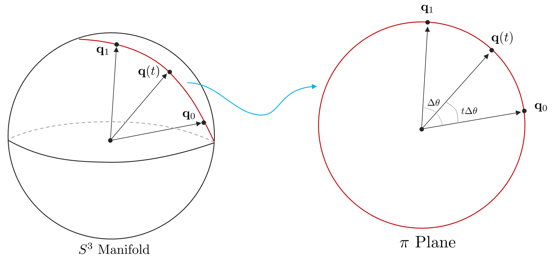
Method 2 다른 구의 선형보간 방법은 쿼터니언 대수학을 사용하거나 manifold에 종속되지 않는 방법이다. 위 그림에서 보면 ${\mathbf{q}}_0,{\mathbf{q}}_1$은 단위 원 내에 존재하는 단위벡터로 볼 수 있다. 보간함수 $\mathbf{q}(t)$는 ${\mathbf{q}}_0$와 ${\mathbf{q}}_1$의 최단거리를 동일한 각속도로 움직이는 단위벡터로 생각할 수 있다. 최단거리는 두 지점을 포함하는 하나의 평면 호(planar arc)를 형성하는데 이를 $\pi$ 평면이라고 정의한다.

첫 번째 접근 방법은 두 단위벡터 ${\mathbf{q}}_0,{\mathbf{q}}_1$ 사이의 각도를 대수학적으로 구하는 것이다.
$$\begin{array}{}\text{(137)}& \cos (\mathrm{\Delta }\theta )={\mathbf{q}}_0^{⊺}{\mathbf{q}}_1\mathrm{\Delta }\theta =\arccos ({\mathbf{q}}_0^{⊺}{\mathbf{q}}_1)\end{array}$$

다음으로 $\pi$ 평면 내에서 두 개의 직교하는 basis $\{{\mathbf{q}}_0,{\mathbf{q}}_{\perp ]}\}$를 정의한다. ${\mathbf{q}}_{\perp }$는 ${\mathbf{q}}_1$를 ${\mathbf{q}}_0$에 대해 직교화한 basis 벡터를 의미한다.
$$\begin{array}{}\text{(138)}& {\mathbf{q}}_{\perp }=\frac{{\mathbf{q}}_1-({\mathbf{q}}_0^{⊺}{\mathbf{q}}_1){\mathbf{q}}_0}{\Vert {\mathbf{q}}_1-({\mathbf{q}}_0^{⊺}{\mathbf{q}}_1){\mathbf{q}}_0\Vert }\end{array}$$

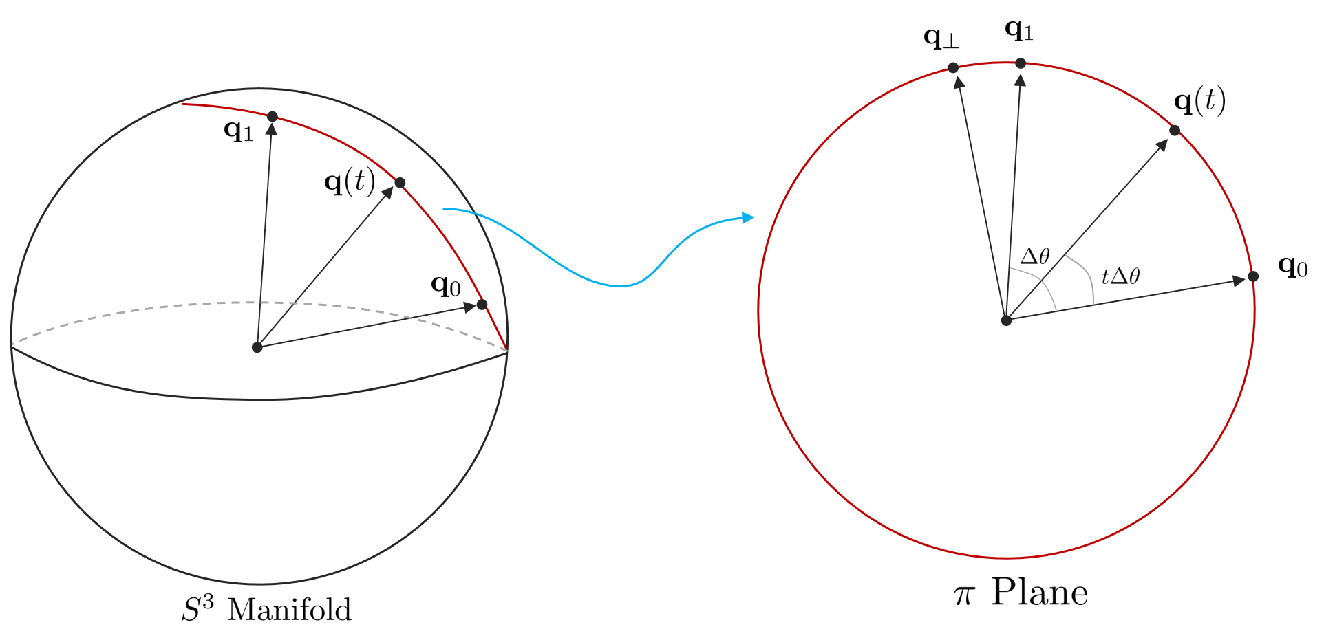
따라서 ${\mathbf{q}}_1$은 다음과 같이 나타낼 수 있다.
$$\begin{array}{}\text{(139)}& {\mathbf{q}}_1={\mathbf{q}}_0\cos \mathrm{\Delta }\theta +{\mathbf{q}}_{\perp }\sin \mathrm{\Delta }\theta \end{array}$$

따라서 보간함수 $\mathbf{q}(t)$는 ${\mathbf{q}}_0$를 $\pi$ 평면을 따라 각도 $t\mathrm{\Delta }\theta$만큼 움직이는 함수가 된다.
$$\begin{array}{}\text{(140)}& \boxed{{\displaystyle \mathbf{q}(t)={\mathbf{q}}_0\cos (t\mathrm{\Delta }\theta )+{\mathbf{q}}_{\perp }\sin (t\mathrm{\Delta }\theta )}}\end{array}$$

Method 3 이와 유사한 방법으로 Glenn Davis in Shoemake (1985)가 제안한 방법이 있다. 이 방법은 ${\mathbf{q}}_0,{\mathbf{q}}_1$이 속한 $\pi$ 평면 내에 임의의 벡터는 선형조합(linear combination)을 통해 나타낼 수 있는 성질을 활용한다. $\mathrm{\Delta }\theta$를 ($\text{137}$)을 통해 계산하고 ${\mathbf{q}}_{\perp }$를 ($\text{139}$)을 통해 구한 후 ($\text{140}$)에 넣으면 다음과 같다. 이 때, $\sin (\mathrm{\Delta }\theta -t\mathrm{\Delta }\theta )=\sin \mathrm{\Delta }\theta \cos t\mathrm{\Delta }\theta -\cos \mathrm{\Delta }\theta \sin t\mathrm{\Delta }\theta$의 성질을 활용함으로써 Davis's formula를 얻을 수 있다.
$$\begin{array}{}\text{(141)}& \boxed{{\displaystyle \mathbf{q}(t)={\mathbf{q}}_0\frac{\sin ((1-t)\mathrm{\Delta }\theta )}{\sin (\mathrm{\Delta }\theta )}+{\mathbf{q}}_1\frac{\sin (t\mathrm{\Delta }\theta )}{\sin \mathrm{\Delta }\theta }}}\end{array}$$

위 식을 $s=1-t$과 같이 치환하여 표현하면 다음과 같은 대칭성을 가진다.
$$\begin{array}{}\text{(142)}& \mathbf{q}(s)={\mathbf{q}}_1\frac{\sin ((1-s)\mathrm{\Delta }\theta )}{\sin (\mathrm{\Delta }\theta )}+{\mathbf{q}}_0\frac{\sin (s\mathrm{\Delta }\theta )}{\sin (\mathrm{\Delta }\theta )}\end{array}$$

이는 위 공식과 ${\mathbf{q}}_0,{\mathbf{q}}_1$이 바뀐 것을 제외하고 정확히 동일하다.

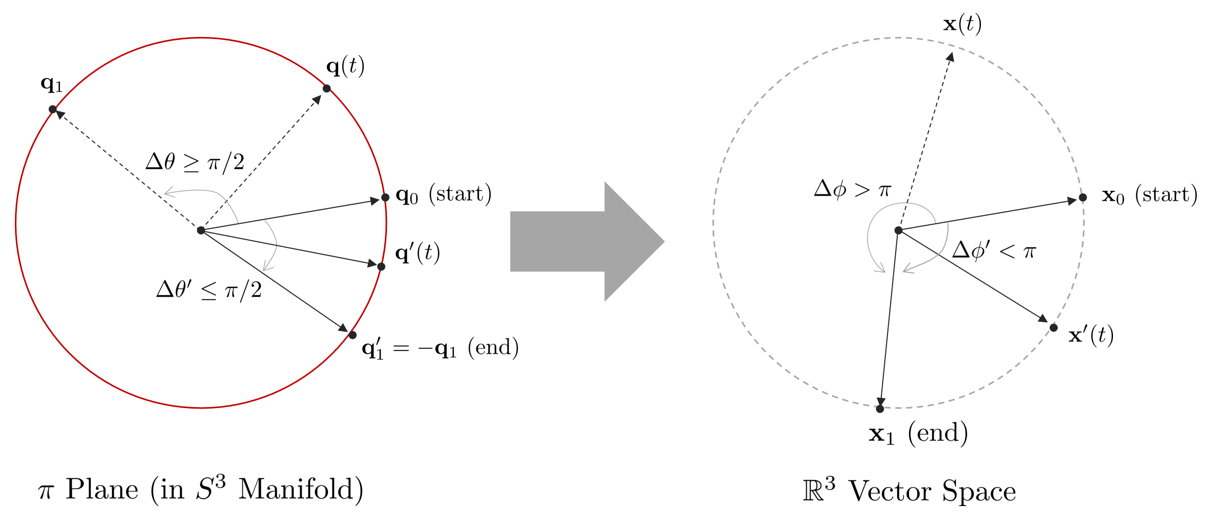
앞서 소개한 모든 쿼터니언 기반의 구의 선형보간 방법들(SLERPs)들은 보간하는 실제 회전각도가 $\varphi \le \pi$와 같은 조건을 가진다. 하지만 이전 챕터에서 설명한 쿼터니언의 SO(3) double cover 성질에 의해, 실제 단위 쿼터니언 공간에서 수행되는 보간은 $\mathrm{\Delta }\theta \le \pi /2$를 만족해야 한다. 따라서 만약 $\cos (\mathrm{\Delta }\theta )={\mathbf{q}}_0^{⊺}{\mathbf{q}}_1<0$이면 ${\mathbf{q}}_1$을 $-{\mathbf{q}}_1$로 치환한 후 보간을 수행한다.

2.8 Quaternion and isoclinic rotations: explaining the magic

본 섹션에서는 다음 두 질문에 대한 답변을 제시한다. Joan Solà는 이를 마법(magic)이라고 부른다.

• 왜 $\mathbf{q}\otimes \mathbf{x}\otimes {\mathbf{q}}^{\ast }$ 연산이 벡터 $\mathbf{x}$를 회전하는 공식이 되는가?
• 왜 쿼터니언을 생성할 때 회전하고자 하는 각도의 절반의 각도를 입력해야 하는가? $\mathbf{q}=e^{\varphi /2}=[\cos \varphi /2,\mathbf{u}\sin \varphi /2]?$
  
  

위 질문에 답을 하기 위해서는 대수적으로 단위 쿼터니언 곱이 벡터의 회전이라는 것을 증명한 ($\text{116}$) 이상의 기하학적인 설명이 필요하다. ($\text{123}$)을 다시 보면 다음과 같다.
$$\begin{array}{}\text{(143)}& \mathbf{q}\otimes \mathbf{x}\otimes {\mathbf{q}}^{\ast }=[{\mathbf{q}}^{\ast }{]}_R[\mathbf{q}{]}_L\left[\begin{array}{c}0\\ \mathbf{x}\end{array}\right]=\left[\begin{array}{c}0\\ \mathbf{Rx}\end{array}\right]\end{array}$$

단위 쿼터니언 $\mathbf{q}$은 다음 두 성질을 만족한다.
$$\begin{array}{}\text{(144)}& \begin{array}{rl}& [\mathbf{q}][\mathbf{q}{]}^{⊺}={\mathbf{I}}_4\\ & det([\mathbf{q}])=+1\end{array}\end{array}$$

이는 SO(4)의 성질과 동일하다. 즉, 단위 쿼터니언은 ${\mathbb{R}}^4$ 공간에서 회전행렬을 의미한다. 구체적으로 말하면, 단위 쿼터니언의 곱은 ${\mathbb{R}}^4$ 공간에서 등복각회전(isoclinic rotation)을 수행한다. 따라서 ($\text{123}$)은 ${\mathbb{R}}^4$ 공간에서 $\mathbf{x}$가 2번의 등복각회전을 수행하는 것을 의미한다. 등복각회전을 이해하기 위해서는 우선 ${\mathbb{R}}^4$ 공간에서 일반적인 회전을 이해해야 한다.

다음은 양영욱님의 저서 수학으로 시작하는 3D 게임 개발에 회전 관련 챕터 내용을 주로 참고하여 작성하였다. 2차원 ${\mathbb{R}}^2$ 공간에서 회전은 점을 중심으로 회전한다. 그리고 3차원 ${\mathbb{R}}^3$ 공간에서 회전은 선을 중심으로 회전한다. 두 차원에서 회전의 공통점이 있다면 점들은 회전하면서 반드시 원을 그린다 사실이다. ${\mathbb{R}}^2$ 공간에서는 이러한 원들이 모두 한 평면 공간상에 존재하지만 ${\mathbb{R}}^3$ 공간에서는 서로 평행한 여러 평면에 존재한다.

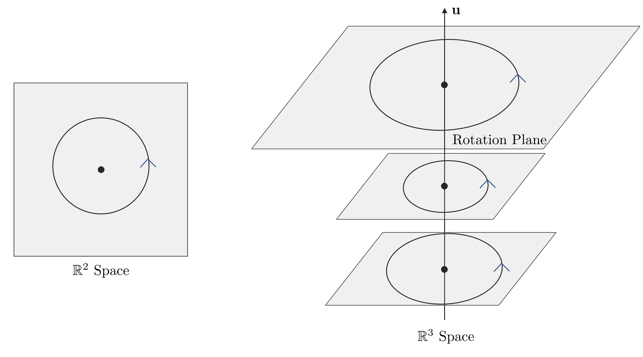
어느 차원에서든 점이 회전하면 당연히 원이 그려지며 그 원이 존재하는 평면이 있게 된다. 따라서 회전을 점이나 선을 기준으로 하지 않고 특정 면을 기준으로 보면 차원과 상관없이 회전을 정의할 수 있으며 이러한 평면을 회전평면(rotation plane)이라고 부른다. 회전이 성립하려면 우선 2차원의 면이 존재해야하므로 1차원에서는 회전이 불가능함을 알 수 있다. ${\mathbb{R}}^2$ 공간에서는 2차원 회전평면을 제외하면 0차원 (2차원-2차원)이 남기 때문에 점을 중심으로 회전한다고 볼 수 있고 ${\mathbb{R}}^3$ 공간에서는 2차원 회전평면을 제외한 1차원 (3차원-2차원)이 남기 때문에 선을 중심으로 회전한다고 볼 수 있다. 따라서 이를 확장하면 ${\mathbb{R}}^4$ 공간에서는 2차원 회전평면을 제외하면 2차원 (4차원-2차원)이 남기 때문에 ${\mathbb{R}}^4$ 공간에서 회전은 면을 중심으로 회전한다는 것을 알수 있다.

하지만 우리는 ${\mathbb{R}}^4$ 공간에서 면을 중심으로 회전하는 것을 쉽게 생각할 수 없으므로 이를 2차원 면이 아닌 1차원의 회전축 2개를 중심으로 회전한다고 생각해볼 수 있다. 그렇다면 각각의 회전축과 수직을 이루는 회전평면 2개를 생각할 수 있다. 즉, ${\mathbb{R}}^4$ 공간에서 회전은 회전평면 ${\pi }_A,{\pi }_B$ 상에서 각각 $\alpha ,\beta$ 각만큼 2개의 회전동시에 일어난다고 볼 수 있다. 이 때, ${\pi }_A,{\pi }_B$ 평면은 서로 직교(orthogonal)하며 이런 회전을 이중회전(double rotation)이라고 부른다. 만약 회전각 $\alpha ,\beta$가 같다면 특별히 이를 등복각 회전(isoclinic rotation)이라고 부른다.

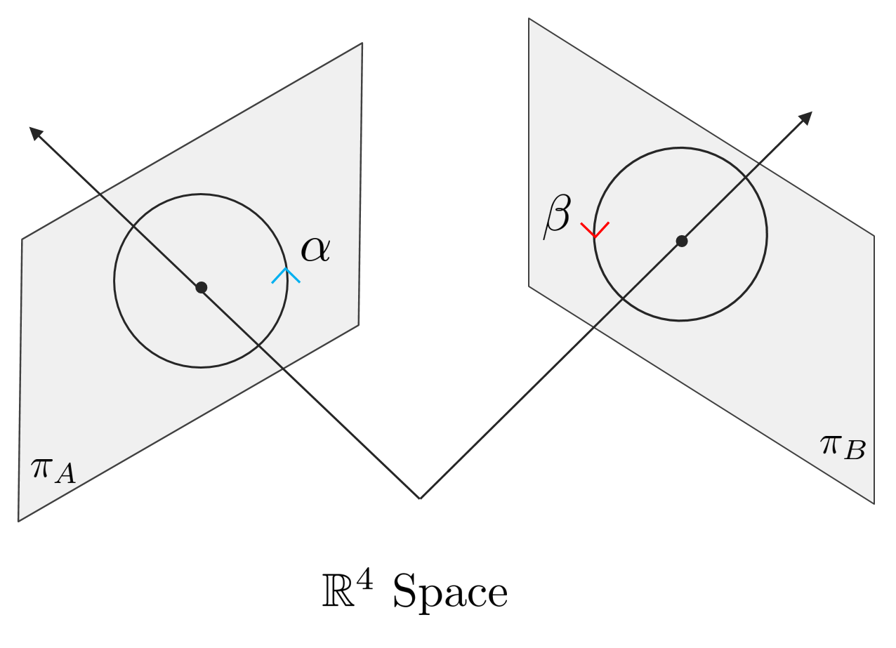
앞서 소개한 단위 쿼터니언 $\mathbf{q}$의 곱은 이러한 ${\mathbb{R}}^4$ 공간에서 등복각 회전을 의미하며 따라서 $\mathbf{q}$를 곱하는 것의 기하학적 의미는 ${\mathbb{R}}^4$ 공간에 존재하는 두 개의 회전평면 ${\pi }_A,{\pi }_B$에서 $\theta$만큼 동시에 두 회전이 일어나게 되는 것을 말한다. 흥미로운 점은 이러한 두 개의 회전평면 ${\pi }_A,{\pi }_B$ 중 하나의 회전평면은 쿼터니언의 벡터를 이루는 $i,j,k$축을 중심으로 회전하는 3차원 공간의 회전평면이라는 사실이다. 따라서 우리는 3차원 공간 상에서 순수 쿼터니언(pure quaternion)으로 변형된 벡터 $\mathbf{x}$가 회전하는 것을 원하므로 하나의 회전평면에서만 회전이 일어나게끔 해야한다.

등복각 회전에는 왼쪽 등복각(left-isoclinic) 회전과 오른쪽 등복각(right-isoclinic) 회전이 존재한다. 왼쪽 등복각 회전은 단위 쿼터니언을 왼쪽에서 곱했을 때 나타나고 오른쪽 등복각 회전은 오른쪽에서 곱했을 때 나타난다.
$$\begin{array}{}\text{(145)}& \begin{array}{rl}& \mathbf{q}\otimes \mathbf{x}:\text{Left isoclinic rotation}\\ & \mathbf{x}\otimes \mathbf{q}:\text{Right isoclinic rotation}\end{array}\end{array}$$

이 때, 두 회전의 곱셈은 교환법칙을 만족한다.
$$\begin{array}{}\text{(146)}& [\mathbf{q}{]}_R[\mathbf{q}{]}_L=[\mathbf{q}{]}_L[\mathbf{q}{]}_R\end{array}$$

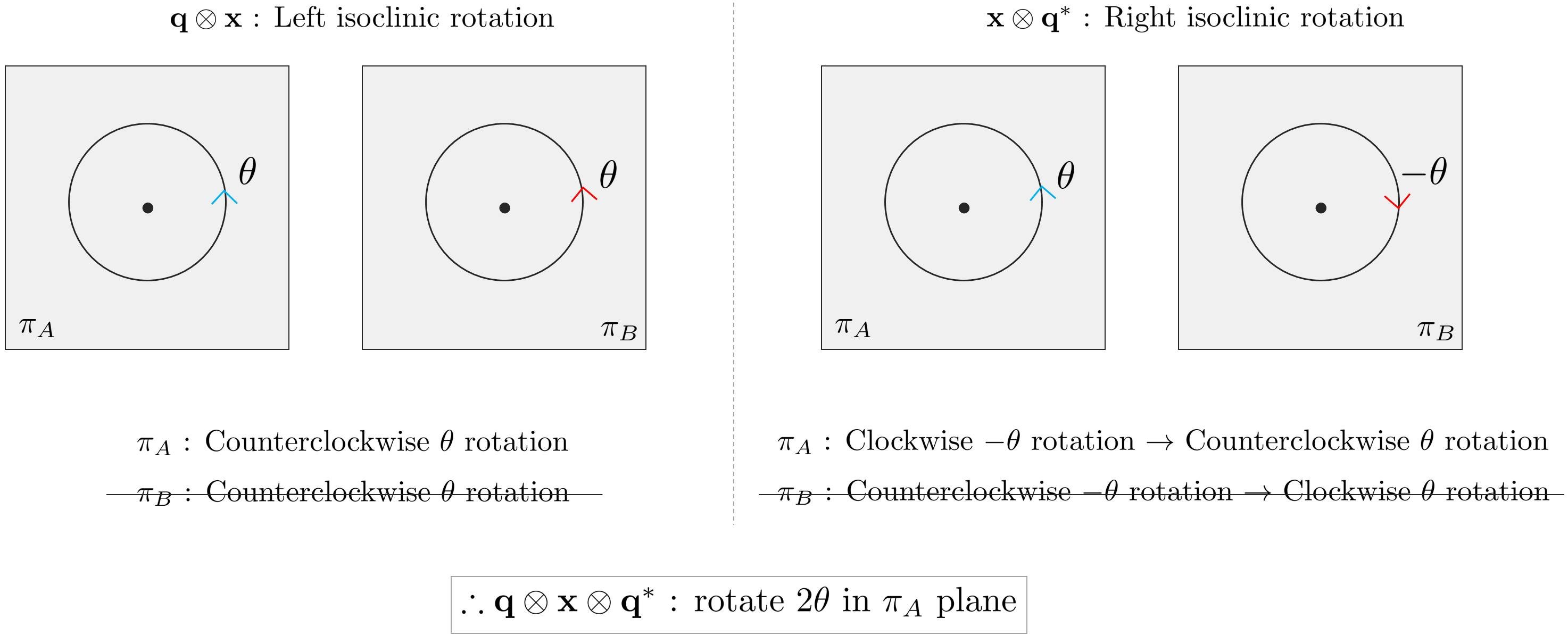
i,j,k 축이 이루는 3차원의 회전평면을 ${\pi }_A$라고 하고 나머지 회전평면을 ${\pi }_B$라고 했을 때, 실제 벡터가 회전하려면 ${\pi }_A$에서만 회전이 일어나고 ${\pi }_B$에서는 회전이 발생하면 안된다. 왼쪽 등복각 회전은 ${\pi }_A$에서 반시계 방향 회전이 일어나고 ${\pi }_B$에서도 반시계 방향 회전이 일어나는 반면, 오른쪽 등복각 회전은 ${\pi }_A$에서 시계방향 회전이 일어나고 ${\pi }_B$에서 시계방향 회전이 일어난다. 즉, ${\pi }_A$는 단위 쿼터니언을 곱하는 방향에 따라 회전의 방향이 바뀌지만 ${\pi }_B$에서는 방향에 상관없이 항상 같은 방향의 회전이 일어난다. 따라서 단위 쿼터니언을 양쪽에 곱하면 ${\pi }_A$ 평면의 회전은 상쇄되어 없어지고 ${\pi }_B$ 평면 상의 회전만 반시계 방향으로 연달아 두 번 하는 것과 동일한 효과를 얻는다.

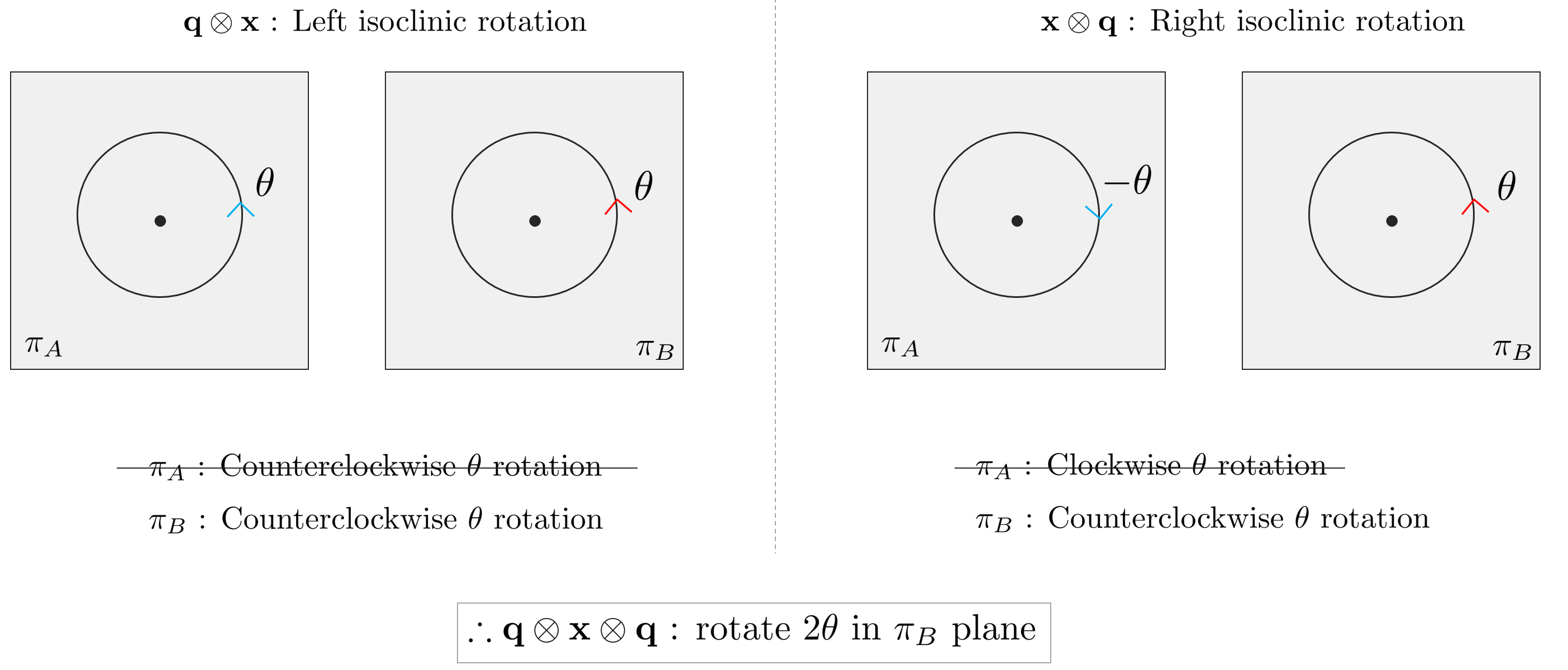
하지만 우리의 목적은 ${\pi }_A$에서만 회전이 일어나는 것을 원하므로 오른쪽 등복각 회전에 반대 방향의 단위 쿼터니언 ${\mathbf{q}}^{\ast }$을 곱해줌으로써 ${\pi }_B$ 평면의 회전을 상쇄시켜줌과 동시에 ${\pi }_A$에 $2\theta$만큼 회전을 수행할 수 있다. 이러한 기하학적 이유로 인해 단위 쿼터니언의 곱이 $\mathbf{q}\otimes \mathbf{x}\otimes {\mathbf{q}}^{\ast }$가 된다.
$$\begin{array}{}\text{(147)}& \left[\begin{array}{c}0\\ {\mathbf{x}}^{\prime }\end{array}\right]=\mathbf{q}\otimes \mathbf{x}\otimes {\mathbf{q}}^{\ast }=[{\mathbf{q}}^{\ast }{]}_R[\mathbf{q}{]}_L\left[\begin{array}{c}0\\ \mathbf{x}\end{array}\right]\end{array}$$

단위 쿼터니언 곱은 하나의 동등한 ${\mathbf{R}}_4$ 행렬로 나타낼수 있다.
$$\begin{array}{}\text{(148)}& {\mathbf{R}}_4\triangleq [{\mathbf{q}}^{\ast }{]}_R[\mathbf{q}{]}_L=[\mathbf{q}{]}_L[{\mathbf{q}}^{\ast }{]}_R=\left[\begin{array}{cc}1& \mathbf{0}\\ \mathbf{0}& \mathbf{R}\end{array}\right]\end{array}$$

이 때, $\mathbf{R}$는 ${\mathbb{R}}^3$ 공간에서 회전행렬을 의미하며 ${\mathbf{R}}_4$는 ${\mathbb{R}}^4$의 부분공간인 ${\mathbb{R}}^3$ 공간 내의 벡터를 회전시키는 행렬이 된다.

References

[1] Sola, Joan. "Quaternion kinematics for the error-state Kalman filter." arXiv preprint arXiv:1711.02508 (2017).