[SLAM] 에러와 자코비안 정리(Errors and Jacobians) 정리 Part 1

arXiv preprint

English version

Notes on Various Errors and Jacobian Derivations for SLAM

 

1. Introduction

본 포스트에서는 SLAM에서 사용하는 다양한 에러에 대한 정의 및 이를 최적화하기 위해 사용하는 자코비안에 대해 설명한다.

 

본 포스트에서 다루는 에러는 다음과 같다.

• Reprojection error $$\begin{array}{}\text{(1)}& \begin{array}{rl}\mathbf{e}& =\mathbf{p}-\hat{\mathbf{p}}\in {\mathbb{R}}^2\end{array}\end{array}$$
• Photometric error $$\begin{array}{}\text{(2)}& \begin{array}{rl}\mathbf{e}& ={\mathbf{I}}_1({\mathbf{p}}_1)-{\mathbf{I}}_2({\mathbf{p}}_2)\in {\mathbb{R}}^1\end{array}\end{array}$$
• Relative pose error  $$\begin{array}{}\text{(3)}& \begin{array}{r}{\mathbf{e}}_{ij}=\text{Log}({\mathbf{z}}_{ij}^{-1}{\hat{\mathbf{z}}}_{ij})\in {\mathbb{R}}^6\end{array}\end{array}$$ 
• Line reprojection error $$\begin{array}{}\text{(4)}& \begin{array}{r}{\mathbf{e}}_l=\left[\begin{array}{cc}\frac{{\mathbf{x}}_s^{⊺}{l}_c}{\sqrt{l_1^2+l_2^2}},& \frac{{\mathbf{x}}_e^{⊺}{l}_c}{\sqrt{l_1^2+l_2^2}}\end{array}\right]\in {\mathbb{R}}^2\end{array}\end{array}$$
  
• IMU measurement error  :  $$\begin{array}{}\text{(5)}& \begin{array}{r}{\mathbf{e}}_{\mathcal{B}}=\left[\begin{array}{c}\delta {\alpha }_{b_{k+1}}^{b_k}\\ \delta {\mathit{\theta }}_{b_{k+1}}^{b_k}\\ \delta {\beta }_{b_{k+1}}^{b_k}\\ \delta {\mathbf{b}}_a\\ \delta {\mathbf{b}}_g\end{array}\right]=\left[\begin{array}{c}{\mathbf{R}}_w^{b_k}({\mathbf{p}}_{b_{k+1}}^w-{\mathbf{p}}_{b_k}^w-{\mathbf{v}}_{b_k}^w\mathrm{\Delta }{t}_k+\frac{1}{2}{\mathbf{g}}^w\mathrm{\Delta }{t}_k^2)-{\hat{\alpha }}_{b_{k+1}}^{b_k}\\ 2[({\hat{\gamma }}_{b_{k+1}}^{b_k}{)}^{-1}\otimes ({\mathbf{q}}_{b_k}^w{)}^{-1}\otimes {\mathbf{q}}_{b_{k+1}}^w{]}_{xyz}\\ {\mathbf{R}}_w^{b_k}({\mathbf{v}}_{b_{k+1}}^w-{\mathbf{v}}_{b_k}^w+{\mathbf{g}}^w\mathrm{\Delta }{t}_k)-{\hat{\beta }}_{b_{k+1}}^{b_k}\\ {\mathbf{b}}_{a_{k+1}}-{\mathbf{b}}_{a_k}\\ {\mathbf{b}}_{g_{k+1}}-{\mathbf{b}}_{g_k}\end{array}\right]\end{array}\end{array}$$
    
  

 

카메라 포즈는 회전행렬 $\mathbf{R}\in SO(3)$로 표현하느냐 또는 변환행렬 $\mathbf{T}\in SE(3)$로 표현하느냐에 따라 서로 다른 자코비안이 유도된다. 두 가지 자코비안을 구하기 위해 reprojection 에러의 경우 SO(3)에 대한 자코비안을 유도하고 photometric 에러의 경우 SE(3)에 대한 자코비안을 유도한다. 또한 3차원 공간 상의 점 또한 $\mathbf{X}=[X,Y,Z,W{]}^{⊺}$로 표현하는 방법과 inverse depth $\rho$로 표현하는 방법에 따라 자코비안이 달라진다. 두 경우에 대한 자코비안 유도 과정에 대해서도 설명한다.

 

본 포스트에서 다루는 자코비안은 다음과 같다. 

• Camera pose (SO(3)-based) $$\begin{array}{}\text{(6)}& \begin{array}{r}\frac{\partial \mathbf{e}}{\partial \mathbf{R}}\to \frac{\partial \mathbf{e}}{\partial \mathrm{\Delta }\mathbf{w}}\end{array}\end{array}$$
• Camera pose (SE(3)-based) $$\begin{array}{}\text{(7)}& \begin{array}{r}\frac{\partial \mathbf{e}}{\partial \mathbf{T}}\to \frac{\partial \mathbf{e}}{\partial \mathrm{\Delta }\xi }\end{array}\end{array}$$
• Map point $$\begin{array}{}\text{(8)}& \begin{array}{r}\frac{\partial \mathbf{e}}{\partial \mathbf{X}}\end{array}\end{array}$$
• Relative pose (SE(3)-based) $$\begin{array}{}\text{(9)}& \begin{array}{rl}& \frac{\partial {\mathbf{e}}_{ij}}{\partial \mathrm{\Delta }{\xi }_i},\frac{\partial {\mathbf{e}}_{ij}}{\partial \mathrm{\Delta }{\xi }_j}\end{array}\end{array}$$ 
• 3D plücker line $$\begin{array}{}\text{(10)}& \begin{array}{rl}& \frac{\partial {\mathbf{e}}_l}{\partial l},\frac{\partial l}{\partial {\mathcal{L}}_c},\frac{\partial {\mathcal{L}}_c}{\partial {\mathcal{L}}_w},\frac{\partial {\mathcal{L}}_w}{\partial {\delta }_{\mathit{\theta }}}\end{array}\end{array}$$  
• Quaternion representation $$\begin{array}{}\text{(11)}& \begin{array}{rl}& \frac{\partial {\mathbf{X}}^{\prime }}{\partial \mathbf{q}}\end{array}\end{array}$$  
• Camera intrinsics $$\begin{array}{}\text{(12)}& \begin{array}{rl}& \frac{\partial \mathbf{e}}{\partial f_x},\frac{\partial \mathbf{e}}{\partial f_y},\frac{\partial \mathbf{e}}{\partial c_x},\frac{\partial \mathbf{e}}{\partial c_y}\end{array}\end{array}$$  
• Inverse depth  $$\begin{array}{}\text{(13)}& \begin{array}{r}\frac{\partial \mathbf{e}}{\partial \rho }\end{array}\end{array}$$  
• IMU error-state system kinematics : $$\begin{array}{}\text{(14)}& \begin{array}{r}{\mathbf{J}}_{b_{k+1}}^{b_k}\end{array}\end{array}$$
• IMU measurement : $$\begin{array}{}\text{(15)}& \begin{array}{r}\frac{\partial {\mathbf{e}}_{\mathcal{B}}}{\partial [{\mathbf{p}}_{b_k}^w,{\mathbf{q}}_{b_k}^w]},\frac{\partial {\mathbf{e}}_{\mathcal{B}}}{\partial [{\mathbf{v}}_{b_k}^w,{\mathbf{b}}_{a_k},{\mathbf{b}}_{g_k}]},\frac{\partial {\mathbf{e}}_{\mathcal{B}}}{\partial [{\mathbf{p}}_{b_{k+1}}^w,{\mathbf{q}}_{b_{k+1}}^w]},\frac{\partial {\mathbf{e}}_{\mathcal{B}}}{\partial [{\mathbf{v}}_{b_{k+1}}^w,{\mathbf{b}}_{a_{k+1}},{\mathbf{b}}_{g_{k+1}}]}\end{array}\end{array}$$

 

2. Optimization formulation

2.1. Error derivation

SLAM에서 에러는 센서 데이터에 의한 관측값(measurement) $\mathbf{z}$과 수학적 모델링에 의한 예측값(estimate) $\hat{\mathbf{z}}$의 차이로 정의한다. 

$$\begin{array}{}\text{(16)}& \boxed{{\displaystyle \begin{array}{r}\mathbf{e}(\mathbf{x})=\mathbf{z}-\hat{\mathbf{z}}(\mathbf{x})\end{array}}}\end{array}$$

- $\mathbf{x}$: 모델의 상태 변수

 

위와 같이 관측값과 예측값의 차이를 에러로 정하고 에러를 최소로 하는 최적의 상태변수 $\mathbf{x}$를 계산하는 것이 SLAM에서 최적화 문제가 된다. 이 때, 일반적인 경우 SLAM의 상태변수에는 회전과 관련된 비선형 항이 포함되므로 비선형 최소제곱법(non-linear least squares) 방법이 주로 사용된다. 

 

2.2. Error function derivation

일반적으로 다량의 센서 데이터가 들어오면 이에 대한 수십~수백개의 에러가 벡터 형태로 계산된다. 이 때, 에러가 정규분포를 따른다고 가정하고 에러 함수로 변환하는 작업을 수행한다. 

$$\begin{array}{}\text{(17)}& \begin{array}{r}\mathbf{e}(\mathbf{x})=\mathbf{z}-\hat{\mathbf{z}}(\mathbf{x})\sim \mathcal{N}(0,\mathbf{\Sigma })\end{array}\end{array}$$

 

에러 함수를 모델링하기 위한 확률변수 $\mathbf{x}$에 대한 다변수 정규분포는 다음과 같다. 
$$\begin{array}{}\text{(18)}& \begin{array}{r}p(\mathbf{x})=\frac{1}{\sqrt{(2\pi {)}^n|\mathbf{\Sigma }|}}\exp (-\frac{1}{2}(\mathbf{x}-\mathit{\mu }{)}^{⊺}\mathbf{\Omega }(\mathbf{x}-\mathit{\mu }))\sim \mathcal{N}(\mathit{\mu },\mathbf{\Sigma })\end{array}\end{array}$$
- $\mathbf{x}\in {\mathbb{R}}^n$
- $\mathit{\mu }\in {\mathbb{R}}^n$: mean vector
- $\mathbf{\Sigma }\in {\mathbb{R}}^{n\times n}$: covariance matrix 
- $|\mathbf{\Sigma }|$: determinant of $\mathbf{\Sigma }$
- $\mathbf{\Omega }={\mathbf{\Sigma }}^{-1}$ : information matrix (inverse of covariance matrix)

 

 

에러를 평균이 $0$이고 분산이 $\mathbf{\Sigma }$인 다변수 정규분포로 모델링할 수 있다. 
$$\begin{array}{}\text{(19)}& \begin{array}{r}p(\mathbf{e})=\frac{1}{\sqrt{(2\pi {)}^n|\mathbf{\Sigma }|}}\exp (-\frac{1}{2}(\mathbf{z}-\hat{\mathbf{z}}(\mathbf{x}){)}^{⊺}{\mathbf{\Sigma }}^{-1}(\mathbf{z}-\hat{\mathbf{z}}(\mathbf{x})))\end{array}\end{array}$$

위 식으로부터 다음과 같은 비례식이 성립한다.
$$\begin{array}{}\text{(20)}& \begin{array}{rl}p(\mathbf{e})& \propto \exp (-\frac{1}{2}(\mathbf{z}-\hat{\mathbf{z}}(\mathbf{x}){)}^{⊺}\mathbf{\Omega }(\mathbf{z}-\hat{\mathbf{z}}(\mathbf{x})))\end{array}\end{array}$$

위 식에 log-likelihood를 적용한 $\ln p(\mathbf{e})$는 다음과 같다.
$$\begin{array}{}\text{(21)}& \begin{array}{rl}\ln p(\mathbf{e})& \propto -\frac{1}{2}(\mathbf{z}-\hat{\mathbf{z}}(\mathbf{x}){)}^{⊺}\mathbf{\Omega }(\mathbf{z}-\hat{\mathbf{z}}(\mathbf{x}))\\ & \propto -\frac{1}{2}\mathbf{e}(\mathbf{x}{)}^{⊺}\mathbf{\Omega }\mathbf{e}(\mathbf{x})\end{array}\end{array}$$

 

log-likelihood $\ln p(\mathbf{e})$가 최대가 되는 ${\mathbf{x}}^{\ast }$를 찾으면 다변수 정규분포의 확률이 최대가 된다. 이를 Maximum Liklihood Estimation (MLE)라고 한다. $\ln p(\mathbf{e})$는 앞에 음수(-)가 있으므로 negative log-likelihood가 최소가되는 $\ln p(\mathbf{e})$를 찾으면 다음과 같다.

$$\begin{array}{}\text{(22)}& \begin{array}{rl}{\mathbf{x}}^{\ast }& =\arg max\ln p(\mathbf{e})\\ & =\arg max-\frac{1}{2}\mathbf{e}(\mathbf{x}{)}^{⊺}\mathbf{\Omega }\mathbf{e}(\mathbf{x})\\ & =\arg min\mathbf{e}(\mathbf{x}{)}^{⊺}\mathbf{\Omega }\mathbf{e}(\mathbf{x})\end{array}\end{array}$$

 

단일 에러가 아닌 모든 에러를 더하여 표현하면 다음과 같고 이를 에러 함수 $\mathbf{E}$ 라고 한다. 실제 최적화 문제에서는 단일 에러 ${\mathbf{e}}_i$가 아닌 에러 함수 $\mathbf{E}$를 최소화하는 ${\mathbf{x}}^{\ast }$를 찾는다.

$$\begin{array}{}\text{(23)}& \boxed{{\displaystyle \begin{array}{rl}\mathbf{E}(\mathbf{x})& =\sum _i{\mathbf{e}}_i(\mathbf{x}{)}^{⊺}{\mathbf{\Omega }}_i{\mathbf{e}}_i(\mathbf{x})\\ {\mathbf{x}}^{\ast }& =\arg min\mathbf{E}(\mathbf{x})\end{array}}}\end{array}$$

2.3. Non-linear least squares

최종적으로 풀어야 하는 최적화 수식은 다음과 같다. 

$$\begin{array}{}\text{(24)}& \begin{array}{r}{\mathbf{x}}^{\ast }=\arg min\mathbf{E}(\mathbf{x})=\arg min\sum _i{\mathbf{e}}_i(\mathbf{x}{)}^{⊺}{\mathbf{\Omega }}_i{\mathbf{e}}_i(\mathbf{x})\end{array}\end{array}$$

 

위 공식에서 에러를 최소화하는 최적 파라미터 ${\mathbf{x}}^{\ast }$를 찾아야 한다. 하지만 위 공식은 SLAM에서 일반적으로 회전에 대한  비선형 항을 포함하므로 closed-form solution이 존재하지 않는다. 따라서 비선형 최적화 방법 (Gauss-Newton (GN), Levenberg-Marquardt (LM))을 사용하여 문제를 풀어야 한다.

 

실제 SLAM의 최적화 수식을 유도하는 과정은 크게 두 방법이 존재한다. 첫 번째로 앞서 설명한 것처럼 MLE를 통해 information matrix를 고려하여 ${\mathbf{e}}_i^{⊺}{\mathbf{\Omega }}_i{\mathbf{e}}_i$ 수식을 최적화하는 방법이 있고 두 번째 방법은 확률을 고려하지 않고  최소제곱법 형태로 나타내어 information matrix가 없는 ${\mathbf{e}}_i^{⊺}{\mathbf{e}}_i$ 수식을 최적화를 수행하는 방법이 있다. 본 포스트에서는 확률을 고려한 MLE 방법에 대해 설명한다.

 

예를 들어, GN 방법을 사용해서 해당 문제를 푼다고 가정해보자. 문제를 푸는 순서는 다음과 같다.

 

1. 에러함수를 정의한다
2. 테일러 전개로 근사 선형화한다
3. 1차 미분 후 0으로 설정한다.
4. 이 때 값을 구하고 이를 에러함수에 대입한다
5. 값이 수렴할 때 까지 반복한다.

 

에러함수 $\mathbf{e}$를 자세히 나타내면 $\mathbf{e}(\mathbf{x})$와 같고 이는 로봇의 포즈 벡터 $\mathbf{x}$에 따라 에러함수의 값이 달라지는 것을 의미한다. GN 방법은 $\mathbf{e}(\mathbf{x})$에 반복적(iterative)으로 에러가 감소하는 방향으로 증분량 $\mathrm{\Delta }\mathbf{x}$를 업데이트한다.
$$\begin{array}{}\text{(25)}& \begin{array}{r}\mathbf{e}(\mathbf{x}+\mathrm{\Delta }\mathbf{x}{)}^{⊺}\mathrm{\Omega }\mathbf{e}(\mathbf{x}+\mathrm{\Delta }\mathbf{x})\end{array}\end{array}$$

이 때, $\mathbf{e}(\mathbf{x}+\mathrm{\Delta }\mathbf{x})$를 $\mathbf{x}$ 부근에서 1차 테일러 전개를 사용하면 위 식은 다음과 같이 근사된다.
$$\begin{array}{}\text{(26)}& \begin{array}{rl}\mathbf{e}(\mathbf{x}+\mathrm{\Delta }\mathbf{x}){|}_{\mathbf{x}}& \approx \mathbf{e}(\mathbf{x})+\mathbf{J}(\mathbf{x}+\mathrm{\Delta }\mathbf{x}-\mathbf{x})\\ & =\mathbf{e}(\mathbf{x})+\mathbf{J}\mathrm{\Delta }\mathbf{x}\end{array}\end{array}$$

이 때, $\mathbf{J}=\frac{\partial \mathbf{e}(\mathbf{x}+\mathrm{\Delta }\mathbf{x})}{\partial \mathbf{x}}$이다. 이를 에러함수 전체에 적용하면 아래와 같다.
$$\begin{array}{}\text{(27)}& \begin{array}{r}\mathbf{e}(\mathbf{x}+\mathrm{\Delta }\mathbf{x}{)}^{⊺}\mathrm{\Omega }\mathbf{e}(\mathbf{x}+\mathrm{\Delta }\mathbf{x})\approx (\mathbf{e}(\mathbf{x})+\mathbf{J}\mathrm{\Delta }\mathbf{x}{)}^{⊺}\mathrm{\Omega }(\mathbf{e}(\mathbf{x})+\mathbf{J}\mathrm{\Delta }\mathbf{x})\end{array}\end{array}$$

위 식을 전개한 후 치환하면 아래와 같다.
$$\begin{array}{}\text{(28)}& \begin{array}{rl}& =\underset{\mathbf{c}}{\underbrace{{\mathbf{e}}^{⊺}\mathrm{\Omega }\mathbf{e}}}+2\underset{\mathbf{b}}{\underbrace{{\mathbf{e}}^{⊺}\mathrm{\Omega }\mathbf{J}}}\mathrm{\Delta }\mathbf{x}+\mathrm{\Delta }{\mathbf{x}}^{⊺}\underset{\mathbf{H}}{\underbrace{{\mathbf{J}}^{⊺}\mathrm{\Omega }\mathbf{J}}}\mathrm{\Delta }\mathbf{x}\\ & =\mathbf{c}+2\mathbf{b}\mathrm{\Delta }\mathbf{x}+\mathrm{\Delta }{\mathbf{x}}^{⊺}\mathbf{H}\mathrm{\Delta }\mathbf{x}\end{array}\end{array}$$

위 전체 에러에 적용하면 다음과 같다.
$$\begin{array}{}\text{(29)}& \begin{array}{r}\mathbf{E}(\mathbf{x}+\mathrm{\Delta }\mathbf{x})=\sum _i{\mathbf{e}}_i(\mathbf{x}{)}^{⊺}{\mathrm{\Omega }}_i{\mathbf{e}}_i(\mathbf{x})=\mathbf{c}+2\mathbf{b}\mathrm{\Delta }\mathbf{x}+\mathrm{\Delta }{\mathbf{x}}^{⊺}\mathbf{H}\mathrm{\Delta }\mathbf{x}\end{array}\end{array}$$

$\mathbf{E}(\mathbf{x}+\mathrm{\Delta }\mathbf{x})$은 $\mathrm{\Delta }\mathbf{x}$에 대한 2차식(Quadratic) 형태이고 $\mathbf{H}={\mathbf{J}}^{⊺}\mathrm{\Omega }\mathbf{J}$는 positive definite 행렬이므로 $\mathbf{E}(\mathbf{x}+\mathrm{\Delta }\mathbf{x})$를 1차 미분하여 0으로 설정한 값이 $\mathrm{\Delta }\mathbf{x}$의 극소가 된다.
$$\begin{array}{}\text{(30)}& \begin{array}{r}\frac{\partial \mathbf{E}(\mathbf{x}+\mathrm{\Delta }\mathbf{x})}{\partial \mathrm{\Delta }\mathbf{x}}\approx 2\mathbf{b}+2\mathbf{H}\mathrm{\Delta }\mathbf{x}=0\end{array}\end{array}$$

이를 정리하면 다음과 같은 공식이 도출된다.
$$\begin{array}{}\text{(31)}& \begin{array}{r}\mathbf{H}\mathrm{\Delta }\mathbf{x}=-\mathbf{b}\end{array}\end{array}$$

이렇게 구한 $\mathrm{\Delta }\mathbf{x}=-{\mathbf{H}}^{-1}\mathbf{b}$를 $\mathbf{x}$에 업데이트해준다.
$$\begin{array}{}\text{(32)}& \begin{array}{r}\mathbf{x}\leftarrow \mathbf{x}+\mathrm{\Delta }\mathbf{x}\end{array}\end{array}$$

지금까지 과정을 반복적(iterative)으로 수행하는 알고리즘을 Gauss-Newton 방법이라고 한다. LM 방법은 GN 방법과 비교했을 때 전체적인 프로세스는 동일하나 증분량을 구하는 공식에서 damping factor $\lambda$항이 추가된다.
$$\begin{array}{}\text{(33)}& \boxed{{\displaystyle \begin{array}{rl}& \text{(GN) }\mathbf{H}\mathrm{\Delta }\mathbf{x}=-\mathbf{b}\\ & \text{(LM) }(\mathbf{H}+\lambda \mathbf{I})\mathrm{\Delta }\mathbf{x}=-\mathbf{b}\end{array}}}\end{array}$$

 

3. Reprojection error

Reprojection 에러는 feature-based Visual SLAM에서 주로 사용되는 에러이다. 주로 feature-based method 기반의 visual odometry(VO) 또는 bundle adjustment(BA)를 수행할 때 사용된다. BA에 대한 자세한 내용은 [SLAM] Bundle Adjustment 개념 리뷰 포스트를 참조하면 된다.

 

 

NOMENCLATURE of reprojection error

• $\tilde{\mathbf{p}}={\pi }_h(\cdot ):\left[\begin{array}{c}{X}^{\prime }\\ Y^{\prime }\\ Z^{\prime }\\ 1\end{array}\right]\to \left[\begin{array}{c}{X}^{\prime }/Z^{\prime }\\ Y^{\prime }/Z^{\prime }\\ 1\end{array}\right]=\left[\begin{array}{c}\tilde{u}\\ \tilde{v}\\ 1\end{array}\right]$    
  • 이미지 평면에 프로젝션하기 위해 3차원 공간 상의 점 ${\mathbf{X}}^{\prime }$를 non-homogeneous 변환한 점
• $\hat{\mathbf{p}}={\pi }_k(\cdot )=\tilde{\mathbf{K}}\tilde{\mathbf{p}}=\left[\begin{array}{ccc}f& 0& c_x\\ 0& f& c_y\end{array}\right]\left[\begin{array}{c}\tilde{u}\\ \tilde{v}\\ 1\end{array}\right]=\left[\begin{array}{c}f\tilde{u}+c_x\\ f\tilde{v}+c_y\end{array}\right]=\left[\begin{array}{c}u\\ v\end{array}\right]$
  • 렌즈 왜곡을 보정한 후 이미지 평면에 프로젝션한 점. 만약 왜곡 보정이 입력 단계에서 이미 수행된 경우 ${\pi }_k(\cdot )=\tilde{\mathbf{K}}(\cdot )$이 된다.
• $\mathbf{K}=\left[\begin{array}{ccc}f& 0& c_x\\ 0& f& c_y\\ 0& 0& 1\end{array}\right]$: 카메라 내부(intrinsic) 파라미터 
• $\tilde{\mathbf{K}}=\left[\begin{array}{ccc}f& 0& c_x\\ 0& f& c_y\end{array}\right]$: ${\mathbb{P}}^2\to {\mathbb{R}}^2$로 프로젝션하기 위해 내부 파라미터의 마지막 행을 생략했다.
• $\mathcal{X}=[{\mathcal{T}}_1,\cdots ,{\mathcal{T}}_m,{\mathbf{X}}_1,\cdots ,{\mathbf{X}}_n{]}^{⊺}$: 모델의 상태변수
• $m$ : 카메라 포즈의 개수
• $n$: 3차원 점의 개수
• ${\mathcal{T}}_i=[{\mathbf{R}}_i,{\mathbf{t}}_i]$
• ${\mathbf{e}}_{ij}={\mathbf{e}}_{ij}(\mathcal{X})$: 간략한 표기를 위해 $\mathcal{X}$ 생략하기도 한다
• ${\mathbf{p}}_{ij}$: 관측된(observed) 특정짐의 픽셀 좌표
• ${\hat{\mathbf{p}}}_{ij}$: 예측된(estimated) 특징점의 픽셀 좌표
• ${\mathbf{T}}_i{\mathbf{X}}_j$: Transformation, 3차원 점 ${\mathbf{X}}_j$를 카메라 좌표계 $\{i\}$로 변환, $({\mathbf{T}}_i{\mathbf{X}}_j=\left[\begin{array}{c}{\mathbf{R}}_i{\mathbf{X}}_j+{\mathbf{t}}_i\\ 1\end{array}\right]\in {\mathbb{R}}^{4\times 1})$
  
  • ${\mathbf{X}}^{\prime }=\mathbf{TX}=[X^{\prime },Y^{\prime },Z^{\prime },1{]}^{⊺}=[{\tilde{\mathbf{X}}}^{\prime },1{]}^{⊺}$
• $\oplus$ : SO(3) 회전행렬  $\mathbf{R}$과 3차원 벡터 $\mathbf{t},\mathbf{X}$를 한 번에 업데이트할 수 있는 연산자.
• $\mathbf{J}=\frac{\partial \mathbf{e}}{\partial \mathcal{X}}=\frac{\partial \mathbf{e}}{\partial [\mathcal{T},\mathbf{X}]}$
• $\mathbf{w}={\left[\begin{array}{ccc}{w}_x& w_y& w_z\end{array}\right]}^{⊺}$: 각속도
• $[\mathbf{w}{]}_{\times }=\left[\begin{array}{ccc}0& -w_z& w_y\\ w_z& 0& -w_x\\ -w_y& w_x& 0\end{array}\right]$ : 각속도 $\mathbf{w}$의 반대칭 행렬
• $\text{Exp}(\mathbf{w})=\exp ([\mathbf{w}{]}_{\times })$

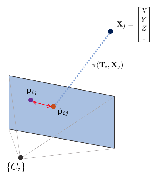
i번째 핀홀카메라 $\{C_i\}$의 포즈 ${\mathbf{T}}_i$와 j번째 월드 상의 한 점 ${\mathbf{X}}_j$가 있을 때 ${\mathbf{X}}_j$는 다음과 같은 변환을 통해 이미지 평면 상에 투영된다.
$$\begin{array}{}\text{(34)}& \begin{array}{r}\text{projection model: }{\hat{\mathbf{p}}}_{ij}=\pi ({\mathbf{T}}_i,{\mathbf{X}}_j)\end{array}\end{array}$$

위와 같이 카메라 내부/외부(intrinsic/extrinsic) 파라미터를 활용한 모델을 projection model이라고 한다. 이를 통한 reprojection 에러는 다음과 같이 정의한다.  

$$\begin{array}{}\text{(35)}& \boxed{{\displaystyle \begin{array}{rl}{\mathbf{e}}_{ij}(\mathcal{X})& ={\mathbf{p}}_{ij}-{\hat{\mathbf{p}}}_{ij}\\ & ={\mathbf{p}}_{ij}-\pi ({\mathbf{T}}_i,{\mathbf{X}}_j)\\ & ={\mathbf{p}}_{ij}-{\pi }_k({\pi }_h({\mathbf{T}}_i{\mathbf{X}}_j))\end{array}}}\end{array}$$

 

모든 카메라 포즈, 3차원 점들에 대한 에러 함수는 다음과 같이 정의된다.

$$\begin{array}{}\text{(36)}& \begin{array}{rl}\mathbf{E}(\mathcal{X})& =\sum _i\sum _j{\Vert {\mathbf{e}}_{ij}(\mathcal{X})\Vert }^2\end{array}\end{array}$$
$$\begin{array}{}\text{(37)}& \begin{array}{rl}{\mathcal{X}}^{\ast }& =\arg \underset{{\mathcal{X}}^{\ast }}{min}\mathbf{E}(\mathcal{X})\\ & =\arg \underset{{\mathcal{X}}^{\ast }}{min}\sum _i\sum _j{\Vert {\mathbf{e}}_{ij}(\mathcal{X})\Vert }^2\\ & =\arg \underset{{\mathcal{X}}^{\ast }}{min}\sum _i\sum _j{\mathbf{e}}_{ij}(\mathcal{X}{)}^{⊺}{\mathbf{e}}_{ij}(\mathcal{X})\\ & =\arg \underset{{\mathcal{X}}^{\ast }}{min}\sum _i\sum _j({\mathbf{p}}_{ij}-{\hat{\mathbf{p}}}_{ij}{)}^{⊺}({\mathbf{p}}_{ij}-{\hat{\mathbf{p}}}_{ij})\end{array}\end{array}$$

 

$\mathbf{E}({\mathcal{X}}^{\ast })$를 만족하는 ${\Vert \mathbf{e}({\mathcal{X}}^{\ast })\Vert }^2$를 non-linear least squares를 통해 반복적으로 계산할 수 있다. 작은 증분량 $\mathrm{\Delta }\mathcal{X}$를 반복적으로 $\mathcal{X}$에 업데이트함으로써 최적의 상태를 찾는다. 
$$\begin{array}{}\text{(38)}& \begin{array}{rl}\arg \underset{{\mathcal{X}}^{\ast }}{min}\mathbf{E}(\mathcal{X}+\mathrm{\Delta }\mathcal{X})& =\arg \underset{{\mathcal{X}}^{\ast }}{min}\sum _i\sum _j{\Vert \mathbf{e}(\mathcal{X}+\mathrm{\Delta }\mathcal{X})\Vert }^2\end{array}\end{array}$$

엄밀하게 말하면 상태 증분량 $\mathrm{\Delta }\mathcal{X}$은 SO(3) 회전행렬을 포함하므로 $\oplus$ 연산자를 통해 기존 상태 $\mathcal{X}$에 더해지는게 맞지만 표현의 편의를 위해 $+$ 연산자를 사용하였다. 

$$\begin{array}{}\text{(39)}& \begin{array}{r}\mathbf{e}(\mathcal{X}\oplus \mathrm{\Delta }\mathcal{X})\to \mathbf{e}(\mathcal{X}+\mathrm{\Delta }\mathcal{X})\end{array}\end{array}$$

 

위 식은 테일러 1차 근사를 통해 다음과 같이 표현이 가능하다.

$$\begin{array}{}\text{(40)}& \begin{array}{rl}\mathbf{e}(\mathcal{X}+\mathrm{\Delta }\mathcal{X})& \approx \mathbf{e}(\mathcal{X})+\mathbf{J}\mathrm{\Delta }\mathcal{X}\\ & =\mathbf{e}(\mathcal{X})+{\mathbf{J}}_c\mathrm{\Delta }\mathcal{T}+{\mathbf{J}}_p\mathrm{\Delta }\mathbf{X}\\ & =\mathbf{e}(\mathcal{X})+\frac{\partial \mathbf{e}}{\partial \mathcal{T}}\mathrm{\Delta }\mathcal{T}+\frac{\partial \mathbf{e}}{\partial \mathbf{X}}\mathrm{\Delta }\mathbf{X}\end{array}\end{array}$$

 

$$\begin{array}{}\text{(41)}& \begin{array}{rl}\arg \underset{{\mathcal{X}}^{\ast }}{min}\mathbf{E}(\mathcal{X}+\mathrm{\Delta }\mathcal{X})& \approx \arg \underset{{\mathcal{X}}^{\ast }}{min}\sum _i\sum _j{\Vert \mathbf{e}(\mathcal{X})+\mathbf{J}\mathrm{\Delta }\mathcal{X}\Vert }^2\end{array}\end{array}$$

 

이를 미분하여 최적의 증분량 $\mathrm{\Delta }{\mathcal{X}}^{\ast }$ 값을 구하면 다음과 같다. 자세한 유도 과정은 본 섹션에서는 생략한다. 유도 과정에 대해 자세히 알고 싶으면 이전 섹션을 참조하면 된다.
$$\begin{array}{}\text{(42)}& \begin{array}{rl}& {\mathbf{J}}^{⊺}\mathbf{J}\mathrm{\Delta }{\mathcal{X}}^{\ast }=-{\mathbf{J}}^{⊺}\mathbf{e}\\ & \mathbf{H}\mathrm{\Delta }{\mathcal{X}}^{\ast }=-\mathbf{b}\end{array}\end{array}$$

 

위 식은 선형시스템 $\mathbf{Ax}=\mathbf{b}$ 형태이므로 schur complement, cholesky decomposition과 같은 다양한 선형대수학 테크닉을 사용하여 $\mathrm{\Delta }{\mathcal{X}}^{\ast }$를 구할 수 있다. 이 때, 기존 상태 $\mathcal{X}$ 중 $\mathbf{t},\mathbf{X}$는 선형 벡터 공간에 존재하므로 오른쪽에서 더하는 지 또는 왼쪽에서 더하는 지에 따른 차이가 없지만 회전 행렬 $\mathbf{R}$은 비선형 SO(3)군에 속하므로 오른쪽에 곱하느냐 왼쪽에 곱하느냐에 따라 각각 로컬 좌표계에서 본 포즈를 업데이트할 것 인지(오른쪽) 전역 좌표계에서 본 포즈를 업데이트할 것 인지(왼쪽) 달라지게 된다. Reprojection 에러는 전역 좌표계의 변환 행렬을 업데이트하므로 일반적으로 왼쪽 곱셈 방법을 사용한다.$$\begin{array}{}\text{(43)}& \begin{array}{r}\mathcal{X}\leftarrow \mathcal{X}\oplus \mathrm{\Delta }{\mathcal{X}}^{\ast }\end{array}\end{array}$$

 

$\mathcal{X}$는 $[\mathcal{T},\mathbf{X}]$로 구성되어 있으므로 다음과 같이 풀어 쓸 수 있다. 

$$\begin{array}{}\text{(44)}& \begin{array}{rl}\mathcal{T}\leftarrow \mathcal{T}& \oplus \mathrm{\Delta }{\mathcal{T}}^{\ast }\\ \mathbf{X}\leftarrow \mathbf{X}& \oplus \mathrm{\Delta }{\mathbf{X}}^{\ast }\end{array}\end{array}$$

 

왼쪽 곱셈 $\oplus$ 연산의 정의는 다음과 같다.

$$\begin{array}{}\text{(45)}& \begin{array}{rl}\mathbf{R}\oplus \mathrm{\Delta }{\mathbf{R}}^{\ast }& =\mathrm{\Delta }{\mathbf{R}}^{\ast }\mathbf{R}\\ & =\text{Exp}(\mathrm{\Delta }{\mathbf{w}}^{\ast })\mathbf{R}\cdots \text{ globally updated (left mult)}\\ \mathbf{t}\oplus \mathrm{\Delta }{\mathbf{t}}^{\ast }& =\mathbf{t}+\mathrm{\Delta }{\mathbf{t}}^{\ast }\\ \mathbf{X}\oplus \mathrm{\Delta }{\mathbf{X}}^{\ast }& =\mathbf{X}+\mathrm{\Delta }{\mathbf{X}}^{\ast }\end{array}\end{array}$$

 

3.1. Jacobian of the reprojection error

3.1.1. Jacobian of camera pose

포즈에 대한 자코비안 ${\mathbf{J}}_c$은 다음과 같이 분해할 수 있다.
$$\begin{array}{}\text{(46)}& \begin{array}{rl}{\mathbf{J}}_c=\frac{\partial \mathbf{e}}{\partial \mathcal{T}}& =\frac{\partial }{\partial \mathcal{T}}(\mathbf{p}-\hat{\mathbf{p}})\\ & =\frac{\partial }{\partial \mathcal{T}}(\mathbf{p}-{\pi }_k({\pi }_h({\mathbf{T}}_i{\mathbf{X}}_j)))\\ & =\frac{\partial }{\partial \mathcal{T}}(-{\pi }_k({\pi }_h({\mathbf{T}}_i{\mathbf{X}}_j)))\end{array}\end{array}$$

 

Chain rule을 사용하여 위 식을 정리하면 다음과 같다. 이 때, 편의를 위해 ${\mathbf{T}}_i{\mathbf{X}}_j\to {\mathbf{X}}^{\prime }$로 표기한다.

$$\begin{array}{}\text{(47)}& \begin{array}{rl}{\mathbf{J}}_c& =\frac{\partial \hat{\mathbf{p}}}{\partial \tilde{\mathbf{p}}}\frac{\partial \tilde{\mathbf{p}}}{\partial {\mathbf{X}}^{\prime }}\frac{\partial {\mathbf{X}}^{\prime }}{\partial [\mathbf{w},\mathbf{t}]}\\ & ={\mathbb{R}}^{2\times 3}\cdot {\mathbb{R}}^{3\times 4}\cdot {\mathbb{R}}^{4\times 6}={\mathbb{R}}^{2\times 6}\end{array}\end{array}$$

 

이 때, 회전행렬 $\mathbf{R}$에 대한 자코비안 $\frac{\partial {\mathbf{X}}^{\prime }}{\partial \mathbf{R}}$을 구하는 것이 아닌 각속도 $\mathbf{w}$에 대한 자코비안 $\frac{\partial {\mathbf{X}}^{\prime }}{\partial \mathbf{w}}$을 구하는 이유는 다음 섹션에서 설명한다.또한 에러를 $\mathbf{p}-\hat{\mathbf{p}}$로 정의하느냐 $\hat{\mathbf{p}}-\mathbf{p}$로 정의하느냐에 따라 ${\mathbf{J}}_c$의 부호 또한 변경되므로 이는 실제 코드로 구현할 때 유의하여 적용해야 한다. 해당 자료에서는 부호는 $+$로 간주하고 표기하였다.

 

렌즈에 의한 왜곡(distortion)은 일반적으로 계산의 복잡성으로 인해 자코비안 계산 시 고려하지 않는다. 또한 렌즈 왜곡 보정(undistortion)이 이미지 입력 과정에서 이미 수행되었다고 가정하면 이를 고려할 필요가 없어진다.

따라서 $\frac{\partial \hat{\mathbf{p}}}{\partial \tilde{\mathbf{p}}}$은 다음과 같이 단순히 카메라 내부 행렬 $\mathbf{K}$를 곱하는 것으로 구할 수 있다. 아래 수식에서는 마지막 행 $[001]$을 생략한 $\tilde{\mathbf{K}}$가 사용되었다.
$$\begin{array}{}\text{(48)}& \boxed{{\displaystyle \begin{array}{rl}\frac{\partial \hat{\mathbf{p}}}{\partial \tilde{\mathbf{p}}}& =\frac{\partial }{\partial \tilde{\mathbf{p}}}\tilde{\mathbf{K}}\tilde{\mathbf{p}}\\ & =\tilde{\mathbf{K}}\\ & =\left[\begin{array}{ccc}f& 0& c_x\\ 0& f& c_y\end{array}\right]\in {\mathbb{R}}^{2\times 3}\end{array}}}\end{array}$$

다음으로 $\frac{\partial \tilde{\mathbf{p}}}{\partial {\mathbf{X}}^{\prime }}$은 다음과 같다.
$$\begin{array}{}\text{(49)}& \boxed{{\displaystyle \begin{array}{rl}\frac{\partial \tilde{\mathbf{p}}}{\partial {\mathbf{X}}^{\prime }}& =\frac{\partial [\tilde{u},\tilde{v},1]}{\partial [X^{\prime },Y^{\prime },Z^{\prime },1]}\\ & =\left[\begin{array}{cccc}\frac{1}{Z^{\prime }}& 0& \frac{-X^{\prime }}{Z^{\prime 2}}& 0\\ 0& \frac{1}{Z^{\prime }}& \frac{-Y^{\prime }}{Z^{\prime 2}}& 0\\ 0& 0& 0& 0\end{array}\right]\in {\mathbb{R}}^{3\times 4}\end{array}}}\end{array}$$

 

다음으로 $\frac{\partial {\mathbf{X}}^{\prime }}{\partial \mathbf{t}}$를 구해야 한다. 이는 다음과 같이 비교적 간단하게 구할 수 있다.
$$\begin{array}{}\text{(50)}& \boxed{{\displaystyle \begin{array}{rl}\frac{\partial {\mathbf{X}}^{\prime }}{\partial \mathbf{t}}& =\frac{\partial }{\partial [t_x,t_y,t_z]}\left[\begin{array}{c}\mathbf{R}\mathbf{X}+\mathbf{t}\\ 1\end{array}\right]\\ & =\frac{\partial }{\partial [t_x,t_y,t_z]}\left[\begin{array}{c}\mathbf{t}\\ 1\end{array}\right]\\ & =\frac{\partial }{\partial [t_x,t_y,t_z]}(\left[\begin{array}{c}{t}_x\\ t_y\\ t_z\\ 1\end{array}\right])\\ & =\left[\begin{array}{ccc}1& 0& 0\\ 0& 1& 0\\ 0& 0& 1\\ 0& 0& 0\end{array}\right]\in {\mathbb{R}}^{4\times 3}\end{array}}}\end{array}$$

 

3.1.2. Lie theory-based SO(3) optmization

마지막으로 $\frac{\partial {\mathbf{X}}^{\prime }}{\partial \mathbf{w}}$를 구해야 한다.  이 때, 회전 관련 파라미터를 회전행렬 $\mathbf{R}$이 아닌 각속도 $\mathbf{w}$로 표현하였다. 회전행렬 $\mathbf{R}$은 파라미터의 개수가 9개인 반면에 실제 회전에는 3개의 자유도로 제한되므로 over-parameterized 되었다. over-parameterized 표현법의 단점은 다음과 같다.

• 중복되는 파라미터를 계산해야 하기 때문에 최적화 수행 시 연산량이 증가한다.
• 추가적인 자유도로 인해 수치적인 불안정성(numerical instability) 문제가 야기될 수 있다.
• 파라미터가 업데이트될 때마다 항상 제약조건을 만족하는 지 체크해줘야 한다.

 

lie theory를 사용하면 제약조건으로부터 자유롭게 최적화를 수행할 수 있다. 따라서 lie group SO(3) $\mathbf{R}$ 대신 lie algebra so(3) $[\mathbf{w}{]}_{\times }$을 사용하여 제약조건으로부터 자유롭게 파라미터를 업데이트할 수 있게 된다. 이 때, $\mathbf{w}\in {\mathbb{R}}^3$는 각속도 벡터를 의미한다.
$$\begin{array}{}\text{(51)}& \begin{array}{r}\frac{\partial \mathbf{e}}{\partial [\mathbf{R},\mathbf{t}]}\to \frac{\partial \mathbf{e}}{\partial [\mathbf{w},\mathbf{t}]}\end{array}\end{array}$$

 

하지만 ${\mathbf{X}}^{\prime }$에서 $\mathbf{w}$이 바로 보이지 않으므로 ${\mathbf{X}}^{\prime }$를 lie algebra로 표현해야 한다. 이 때, 회전과 관련된 $\mathbf{w}$ 항에 대한 자코비안을 구해야 하므로 3차원 점 ${\mathbf{X}}_t$를 $\mathbf{X}$가 $\mathbf{t}$만큼 병진 이동한 후, ${\mathbf{X}}^{\prime }$를 동일한 위치의 ${\mathbf{X}}_t$가 $\mathbf{R}$만큼 회전한 점이라고 하자.

$$\begin{array}{}\text{(52)}& \begin{array}{rl}{\mathbf{X}}_t& =\mathbf{X}+\mathbf{t}\\ {\mathbf{X}}^{\prime }& =\mathbf{R}{\mathbf{X}}_t\\ & =\text{Exp}(\mathbf{w}){\mathbf{X}}_t\end{array}\end{array}$$

 

$\text{Exp}(\mathbf{w})\in SO(3)$는 각속도 $\mathbf{w}$를 exponential mapping하여 3차원 회전행렬 $\mathbf{R}$로 변환하는 연산을 말한다. exponential mapping에 대한 자세한 내용은 해당 링크를 참조하면 된다. $$\begin{array}{}\text{(53)}& \begin{array}{r}\text{Exp}(\mathbf{w})=\mathbf{R}\end{array}\end{array}$$

 

 

이 때, 작은 lie algebra 증분량 $\mathrm{\Delta }\mathbf{w}$를 기존 $\text{Exp}(\mathbf{w})$에 업데이트하는 방식에 따라 두 가지 방법으로 나뉘게 된다. 우선 $[1]$ 기본적인 lie algebra를 사용한 업데이트 방법이 있다. 다음으로 $[2]$ 섭동(perturbation) 모델을 활용한 업데이트 방법이 있다. 
$$\begin{array}{}\text{(54)}& \begin{array}{rl}\text{Exp}(\mathbf{w})& \leftarrow \text{Exp}(\mathbf{w}+\mathrm{\Delta }\mathbf{w})\cdots \text{[1]}\\ \text{Exp}(\mathbf{w})& \leftarrow \text{Exp}(\mathrm{\Delta }\mathbf{w})\text{Exp}(\mathbf{w})\cdots \text{[2]}\end{array}\end{array}$$

 

위 두 방법 사이에는 다음과 같은 관계가 존재한다. 자세한 내용은 해당 링크의 4.3.3 챕터를 참조하면 된다. $$\begin{array}{}\text{(55)}& \begin{array}{rl}& \text{Exp}(\mathrm{\Delta }\mathbf{w})\text{Exp}(\mathbf{w})=\text{Exp}(\mathbf{w}+{\mathbf{J}}_l^{-1}\mathrm{\Delta }\mathbf{w})\\ & \text{Exp}(\mathbf{w}+\mathrm{\Delta }\mathbf{w})=\text{Exp}({\mathbf{J}}_l\mathrm{\Delta }\mathbf{w})\text{Exp}(\mathbf{w})\end{array}\end{array}$$

 

 

$[1]$ Lie algebra-based update: 우선 $[1]$ 방법을 사용해서 자코비안 $\frac{\partial \mathbf{R}{\mathbf{X}}_t}{\partial \mathbf{w}}$를 바로 계산하면 다음과 같은 복잡한 식이 유도된다.

$$\begin{array}{}\text{(56)}& \boxed{{\displaystyle \begin{array}{rl}\frac{\partial \mathbf{R}{\mathbf{X}}_t}{\partial \mathbf{w}}& =\underset{\mathrm{\Delta }\mathbf{w}\to 0}{lim}\frac{\text{Exp}(\mathbf{w}+\mathrm{\Delta }\mathbf{w}){\mathbf{X}}_t-\text{Exp}(\mathbf{w}){\mathbf{X}}_t}{\mathrm{\Delta }\mathbf{w}}\\ & \approx \underset{\mathrm{\Delta }\mathbf{w}\to 0}{lim}\frac{\text{Exp}({\mathbf{J}}_l\mathrm{\Delta }\mathbf{w})\text{Exp}(\mathbf{w}){\mathbf{X}}_t-\text{Exp}(\mathbf{w}){\mathbf{X}}_t}{\mathrm{\Delta }\mathbf{w}}\\ & \approx \underset{\mathrm{\Delta }\mathbf{w}\to 0}{lim}\frac{(\mathbf{I}+[{\mathbf{J}}_l\mathrm{\Delta }\mathbf{w}{]}_{\times })\text{Exp}(\mathbf{w}){\mathbf{X}}_t-\text{Exp}(\mathbf{w}){\mathbf{X}}_t}{\mathrm{\Delta }\mathbf{w}}\\ & =\underset{\mathrm{\Delta }\mathbf{w}\to 0}{lim}\frac{[{\mathbf{J}}_l\mathrm{\Delta }\mathbf{w}{]}_{\times }\mathbf{R}{\mathbf{X}}_t}{\mathrm{\Delta }\mathbf{w}}(\because \text{Exp}(\mathbf{w}){\mathbf{X}}_t=\mathbf{R}{\mathbf{X}}_t)\\ & =\underset{\mathrm{\Delta }\mathbf{w}\to 0}{lim}\frac{-[\mathbf{R}{\mathbf{X}}_t{]}_{\times }{\mathbf{J}}_l\mathrm{\Delta }\mathbf{w}}{\mathrm{\Delta }\mathbf{w}}\\ & =-[\mathbf{R}{\mathbf{X}}_t{]}_{\times }{\mathbf{J}}_l\\ & =-[{\mathbf{X}}^{\prime }{]}_{\times }{\mathbf{J}}_l\end{array}}}\end{array}$$

 

위 식에서 두 번째 행은 BCH 근사를 사용하여 왼쪽 자코비안(left jacobian) ${\mathbf{J}}_l$이 유도된 형태이고 세 번째 행은 작은 회전량 $\text{Exp}({\mathbf{J}}_l\mathrm{\Delta }\mathbf{w})$에 대해 1차 테일러 근사가 적용된 형태이다. ${\mathbf{J}}_l$에 대한 자세한 내용은 Lie theory 개념 리뷰 포스팅을 참조하면 된다.

세 번째 행의 근사를 이해하기 위해 임의의 회전 벡터 $\mathbf{w}=[w_x,w_y,w_z{]}^{⊺}$가 주어졌을 때 회전행렬을 exponential mapping 형태로 전개하면 다음과 같이 나타낼 수 있다. $$\begin{array}{}\text{(57)}& \begin{array}{rl}\mathbf{R}& =\text{Exp}(\mathbf{w})\\ & =\exp ([\mathbf{w}{]}_{\times })\\ & =\mathbf{I}+[\mathbf{w}{]}_{\times }+\frac{1}{2}[\mathbf{w}{]}_{\times }^2+\frac{1}{3!}[\mathbf{w}{]}_{\times }^3+\frac{1}{4!}[\mathbf{w}{]}_{\times }^4+\cdots \end{array}\end{array}$$

작은 크기의 회전행렬 $\mathrm{\Delta }\mathbf{R}$에 대해서는 2차 이상의 고차항을 무시하여 다음과 같이 근사적으로 나타낼 수 있다. $$\begin{array}{}\text{(58)}& \begin{array}{r}\mathrm{\Delta }\mathbf{R}\approx \mathbf{I}+[\mathrm{\Delta }\mathbf{w}{]}_{\times }\end{array}\end{array}$$

$[2]$ Perturbation model-based update: ${\mathbf{J}}_l$을 사용하지 않고 보다 간단한 자코비안을 구하기 위해 $[2]$ lie algebra so(3)의 섭동(perturbation) 모델을 일반적으로 사용한다. 섭동 모델을 사용하여 자코비안 $\frac{\partial \mathbf{R}{\mathbf{X}}_t}{\partial \mathrm{\Delta }\mathbf{w}}$를 구하면 다음과 같다.

$$\begin{array}{}\text{(59)}& \boxed{{\displaystyle \begin{array}{rl}\frac{\partial \mathbf{R}{\mathbf{X}}_t}{\partial \mathrm{\Delta }\mathbf{w}}& =\underset{\mathrm{\Delta }\mathbf{w}\to 0}{lim}\frac{\text{Exp}(\mathrm{\Delta }\mathbf{w})\text{Exp}(\mathbf{w}){\mathbf{X}}_t-\text{Exp}(\mathbf{w}){\mathbf{X}}_t}{\mathrm{\Delta }\mathbf{w}}\\ & \approx \underset{\mathrm{\Delta }\mathbf{w}\to 0}{lim}\frac{(\mathbf{I}+[\mathrm{\Delta }\mathbf{w}{]}_{\times })\text{Exp}(\mathbf{w}){\mathbf{X}}_t-\text{Exp}(\mathbf{w}){\mathbf{X}}_t}{\mathrm{\Delta }\mathbf{w}}\\ & =\underset{\mathrm{\Delta }\mathbf{w}\to 0}{lim}\frac{[\mathrm{\Delta }\mathbf{w}{]}_{\times }\mathbf{R}{\mathbf{X}}_t}{\mathrm{\Delta }\mathbf{w}}(\because \text{Exp}(\mathbf{w}){\mathbf{X}}_t=\mathbf{R}{\mathbf{X}}_t)\\ & =\underset{\mathrm{\Delta }\mathbf{w}\to 0}{lim}\frac{-[\mathbf{R}{\mathbf{X}}_t{]}_{\times }\mathrm{\Delta }\mathbf{w}}{\mathrm{\Delta }\mathbf{w}}\\ & =-[\mathbf{R}{\mathbf{X}}_t{]}_{\times }\\ & =-[{\mathbf{X}}^{\prime }{]}_{\times }\end{array}}}\end{array}$$

 

위 식 또한 두 번째 행에서 작은 회전행렬에 대한 근사 $\text{Exp}(\mathrm{\Delta }\mathbf{w})\approx \mathbf{I}+[\mathrm{\Delta }\mathbf{w}{]}_{\times }$를 사용하였다. 따라서 $[2]$ 섭동 모델을 사용하는 경우 3차원 공간 상의 점 ${\mathbf{X}}^{\prime }$의 반대칭 행렬을 사용하여 간단하게 자코비안 $\frac{\partial \mathbf{R}{\mathbf{X}}_t}{\partial \mathrm{\Delta }\mathbf{w}}$을 구할 수 있는 이점이 있다. reprojection 에러 최적화의 경우 대부분 순차적으로 들어오는 이미지들의 특징점에 대한 에러를 최적화하므로 카메라 포즈 변화가 크지 않고 따라서 $\mathrm{\Delta }\mathbf{w}$의 크기 또한 크지 않으므로 일반적으로 위의 자코비안 $\frac{\partial \mathbf{R}{\mathbf{X}}_t}{\partial \mathrm{\Delta }\mathbf{w}}$을 주로 사용한다. $[2]$ 방법을 사용하므로 기존 회전행렬 $\mathbf{R}$에 작은 증분량 $\mathrm{\Delta }\mathbf{w}$를 업데이트할 때 ($\text{45}$) 같이 업데이트한다.

$$\begin{array}{}\text{(60)}& \begin{array}{r}\mathbf{R}\leftarrow \mathrm{\Delta }{\mathbf{R}}^{\ast }\mathbf{R}\text{where, }\mathrm{\Delta }{\mathbf{R}}^{\ast }=\text{Exp}(\mathrm{\Delta }{\mathbf{w}}^{\ast })\end{array}\end{array}$$

 

따라서 기존의 자코비안은 $\frac{\partial {\mathbf{X}}^{\prime }}{\partial [\mathbf{w},\mathbf{t}]}$에서 $\frac{\partial {\mathbf{X}}^{\prime }}{\partial [\mathrm{\Delta }\mathbf{w},\mathbf{t}]}$로 변경되고 이는 다음과 같다.
$$\begin{array}{}\text{(61)}& \boxed{{\displaystyle \begin{array}{rl}\frac{\partial }{\partial [\mathrm{\Delta }\mathbf{w},\mathbf{t}]}\left[\begin{array}{c}\mathbf{RX}+\mathbf{t}\\ 1\end{array}\right]& =\left[\begin{array}{cccccc}0& Z^{\prime }& -Y^{\prime }& 1& 0& 0\\ -Z^{\prime }& 0& X^{\prime }& 0& 1& 0\\ Y^{\prime }& -X^{\prime }& 0& 0& 0& 1\\ 0& 0& 0& 0& 0& 0\end{array}\right]\in {\mathbb{R}}^{4\times 6}\end{array}}}\end{array}$$

최종적인 포즈에 대한 자코비안 ${\mathbf{J}}_c$는 다음과 같다.
$$\begin{array}{}\text{(62)}& \boxed{{\displaystyle \begin{array}{rl}{\mathbf{J}}_c& =\frac{\partial \hat{\mathbf{p}}}{\partial \tilde{\mathbf{p}}}\frac{\partial \tilde{\mathbf{p}}}{\partial {\mathbf{X}}^{\prime }}\frac{\partial {\mathbf{X}}^{\prime }}{\partial [\mathrm{\Delta }\mathbf{w},\mathbf{t}]}\\ & =\left[\begin{array}{ccc}f& 0& c_x\\ 0& f& c_y\end{array}\right]\left[\begin{array}{cccc}\frac{1}{Z^{\prime }}& 0& \frac{-X^{\prime }}{Z^{\prime 2}}& 0\\ 0& \frac{1}{Z^{\prime }}& \frac{-Y^{\prime }}{Z^{\prime 2}}& 0\\ 0& 0& 0& 0\end{array}\right]\left[\begin{array}{cccccc}0& Z^{\prime }& -Y^{\prime }& 1& 0& 0\\ -Z^{\prime }& 0& X^{\prime }& 0& 1& 0\\ Y^{\prime }& -X^{\prime }& 0& 0& 0& 1\\ 0& 0& 0& 0& 0& 0\end{array}\right]\\ & =\left[\begin{array}{cccc}\frac{f}{Z^{\prime }}& 0& -\frac{fX}{Z^{\prime 2}}& 0\\ 0& \frac{f}{Z^{\prime }}& -\frac{fY}{Z^{\prime 2}}& 0\end{array}\right]\left[\begin{array}{cccccc}0& Z^{\prime }& -Y^{\prime }& 1& 0& 0\\ -Z^{\prime }& 0& X^{\prime }& 0& 1& 0\\ Y^{\prime }& -X^{\prime }& 0& 0& 0& 1\\ 0& 0& 0& 0& 0& 0\end{array}\right]\\ & =\left[\begin{array}{cccccc}-\frac{f{X}^{\prime }{Y}^{\prime }}{Z^{\prime 2}}& \frac{f(1+X^{\prime 2})}{Z^{\prime 2}}& -\frac{f{Y}^{\prime }}{Z^{\prime }}& \frac{f}{Z^{\prime }}& 0& -\frac{f{X}^{\prime }}{Z^{\prime 2}}\\ -\frac{f(1+y^2)}{Z^{\prime 2}}& \frac{f{X}^{\prime }{Y}^{\prime }}{Z^{\prime 2}}& \frac{f{X}^{\prime }}{Z^{\prime }}& 0& \frac{f}{Z^{\prime }}& -\frac{f{Y}^{\prime }}{Z^{\prime 2}}\end{array}\right]\in {\mathbb{R}}^{2\times 6}\end{array}}}\end{array}$$

 

 

3.2. Jacobian of Map Point

3차원 점 $\mathbf{X}$에 대한 자코비안 ${\mathbf{J}}_p$은 다음과 같이 구할 수 있다. 

$$\begin{array}{}\text{(63)}& \begin{array}{rl}{\mathbf{J}}_p=\frac{\partial \mathbf{e}}{\partial \mathbf{X}}& =\frac{\partial }{\partial \mathbf{X}}(\mathbf{p}-\hat{\mathbf{p}})\\ & =\frac{\partial }{\partial \mathbf{X}}(\mathbf{p}-{\pi }_k({\pi }_h({\mathbf{T}}_i{\mathbf{X}}_j)))\\ & =\frac{\partial }{\partial \mathbf{X}}(-{\pi }_k({\pi }_h({\mathbf{T}}_i{\mathbf{X}}_j)))\end{array}\end{array}$$

Chain rule을 사용하여 위 식을 정리하면 다음과 같다. 
$$\begin{array}{}\text{(64)}& \begin{array}{rl}{\mathbf{J}}_p& =\frac{\partial \hat{\mathbf{p}}}{\partial \tilde{\mathbf{p}}}\frac{\partial \tilde{\mathbf{p}}}{\partial {\mathbf{X}}^{\prime }}\frac{\partial {\mathbf{X}}^{\prime }}{\partial \mathbf{X}}\\ & ={\mathbb{R}}^{2\times 3}\cdot {\mathbb{R}}^{3\times 4}\cdot {\mathbb{R}}^{4\times 4}={\mathbb{R}}^{2\times 4}\end{array}\end{array}$$

이 중, $\frac{\partial \hat{\mathbf{p}}}{\partial \tilde{\mathbf{p}}}\frac{\partial \hat{\mathbf{p}}}{\partial {\mathbf{X}}^{\prime }}$는 앞서 구한 자코비안과 동일하다. 따라서 $\frac{\partial {\mathbf{X}}^{\prime }}{\partial \mathbf{X}}$만 계산하면 된다.
$$\begin{array}{}\text{(65)}& \boxed{{\displaystyle \begin{array}{rl}\frac{\partial {\mathbf{X}}^{\prime }}{\partial \mathbf{X}}& =\frac{\partial }{\partial \mathbf{X}}\left[\begin{array}{c}\mathbf{R}\mathbf{X}+\mathbf{t}\\ 1\end{array}\right]\\ & =\left[\begin{array}{c}\mathbf{R}\\ 0\end{array}\right]\end{array}}}\end{array}$$

따라서 ${\mathbf{J}}_p$는 다음과 같다.
$$\begin{array}{}\text{(66)}& \boxed{{\displaystyle \begin{array}{rl}{\mathbf{J}}_p& =\frac{\partial \hat{\mathbf{p}}}{\partial \tilde{\mathbf{p}}}\frac{\partial \tilde{\mathbf{p}}}{\partial {\mathbf{X}}^{\prime }}\frac{\partial {\mathbf{X}}^{\prime }}{\partial \mathbf{X}}\\ & =\left[\begin{array}{ccc}f& 0& c_x\\ 0& f& c_y\end{array}\right]\left[\begin{array}{cccc}\frac{1}{Z^{\prime }}& 0& \frac{-X^{\prime }}{Z^{\prime 2}}& 0\\ 0& \frac{1}{Z^{\prime }}& \frac{-Y^{\prime }}{Z^{\prime 2}}& 0\\ 0& 0& 0& 0\end{array}\right]\left[\begin{array}{c}\mathbf{R}\\ 0\end{array}\right]\\ & =\left[\begin{array}{cccc}\frac{f}{Z^{\prime }}& 0& -\frac{f{X}^{\prime }}{Z^{\prime 2}}& 0\\ 0& \frac{f}{Z^{\prime }}& -\frac{f{Y}^{\prime }}{Z^{\prime 2}}& 0\end{array}\right]\left[\begin{array}{c}\mathbf{R}\\ 0\end{array}\right]\in {\mathbb{R}}^{2\times 4}\end{array}}}\end{array}$$

일반적으로 ${\mathbf{J}}_p$의 마지막 열은 항상 0이므로 이를 생략하여 non-homogeneous 형태로 나타내기도 한다.

$$\begin{array}{}\text{(67)}& \boxed{{\displaystyle \begin{array}{rl}{\mathbf{J}}_p& =\left[\begin{array}{ccc}\frac{f}{Z^{\prime }}& 0& -\frac{f{X}^{\prime }}{Z^{\prime 2}}\\ 0& \frac{f}{Z^{\prime }}& -\frac{f{Y}^{\prime }}{Z^{\prime 2}}\end{array}\right]\mathbf{R}\in {\mathbb{R}}^{2\times 3}\end{array}}}\end{array}$$

 

3.3. Code implementations

• g2o 코드: edge_project_xyz.cpp#L82
• g2o 코드: edge_project_xyz.cpp#L80 

 

4. Photometric error

Phtometric 에러는 direct Visual SLAM에서 주로 사용되는 에러이다. 주로 direct method 기반의 visual odometry(VO) 또는 bundle adjustment(BA)를 수행할 때 사용된다. direct method에 대한 자세한 내용은 [SLAM] Optical Flow와 Direct Method 개념 및 코드 리뷰 포스트를 참조하면 된다.

 

 

NOMENCLATURE of photometric error

• ${\tilde{\mathbf{p}}}_2={\pi }_h(\cdot ):\left[\begin{array}{c}{X}^{\prime }\\ Y^{\prime }\\ Z^{\prime }\\ 1\end{array}\right]\to \left[\begin{array}{c}{X}^{\prime }/Z^{\prime }\\ Y^{\prime }/Z^{\prime }\\ 1\end{array}\right]=\left[\begin{array}{c}{\tilde{u}}_2\\ {\tilde{v}}_2\\ 1\end{array}\right]$    
  • 이미지 평면에 프로젝션하기 위해 3차원 공간 상의 점 ${\mathbf{X}}^{\prime }$를 non-homogeneous 변환한 점
• ${\mathbf{p}}_2={\pi }_k(\cdot )=\tilde{\mathbf{K}}{\tilde{\mathbf{p}}}_2=\left[\begin{array}{ccc}f& 0& c_x\\ 0& f& c_y\end{array}\right]\left[\begin{array}{c}{\tilde{u}}_2\\ {\tilde{v}}_2\\ 1\end{array}\right]=\left[\begin{array}{c}f\tilde{u}+c_x\\ f\tilde{v}+c_y\end{array}\right]=\left[\begin{array}{c}{u}_2\\ v_2\end{array}\right]$
  
  • 렌즈 왜곡을 보정한 후 이미지 평면에 프로젝션한 점. 만약 왜곡 보정이 입력 단계에서 이미 수행된 경우 ${\pi }_k(\cdot )=\tilde{\mathbf{K}}(\cdot )$이 된다.
• $\mathbf{K}=\left[\begin{array}{ccc}f& 0& c_x\\ 0& f& c_y\\ 0& 0& 1\end{array}\right]$: 카메라 내부(intrinsic) 파라미터 
• $\tilde{\mathbf{K}}=\left[\begin{array}{ccc}f& 0& c_x\\ 0& f& c_y\end{array}\right]$: ${\mathbb{P}}^2\to {\mathbb{R}}^2$로 프로젝션하기 위해 내부 파라미터의 마지막 행을 생략했다.
• $\mathcal{P}$:  이미지 내의 모든 특징점들의 집합
• $\mathbf{e}(\mathbf{T})\to \mathbf{e}$: 일반적으로 표기를 생략하여 간단하게 나타내기도 한다. 
• ${\mathbf{p}}_1^i,{\mathbf{p}}_2^i$: 첫번째 이미지와 두번째 이미지에서 i번째 특징점의 픽셀 좌표
• $\oplus$ : 두 SE(3) 군을 결합(composition)하는 연산자
• $\mathbf{J}=\frac{\partial \mathbf{e}}{\partial \mathbf{T}}=\frac{\partial \mathbf{e}}{\partial [\mathbf{R},\mathbf{t}]}$
• ${\mathbf{X}}^{\prime }=[X,Y,Z,1{]}^{⊺}=[\widetilde{{\mathbf{X}}^{\prime }},1{]}^{⊺}=\mathbf{TX}$
• $\mathbf{T}\mathbf{X}$: Transformation, 3차원 점 $\mathbf{X}$를 카메라 좌표계로 변환, $(\mathbf{T}\mathbf{X}=\left[\begin{array}{c}\mathbf{R}\mathbf{X}+\mathbf{t}\\ 1\end{array}\right]\in {\mathbb{R}}^{4\times 1})$
• ${\mathbf{X}}^{\prime }=[X^{\prime },Y^{\prime },Z^{\prime },1{]}^{⊺}=[{\tilde{\mathbf{X}}}^{\prime },1{]}^{⊺}$
• $\xi =[\mathbf{w},\mathbf{v}{]}^{⊺}=[w_x,w_y,w_z,v_x,v_y,v_z{]}^{⊺}$: 3차원 각속도와 속도로 구성된 벡터. twist라고 불린다.
• $[\xi {]}_{\times }=\left[\begin{array}{cc}[\mathbf{w}{]}_{\times }& \mathbf{v}\\ {\mathbf{0}}^{⊺}& 0\end{array}\right]\in \text{se}(3)$ : hat 연산자가 적용된 twist의 lie algebra (4x4 행렬)
• $\text{Exp}(\xi )=\exp ([\xi {]}_{\times })$

 

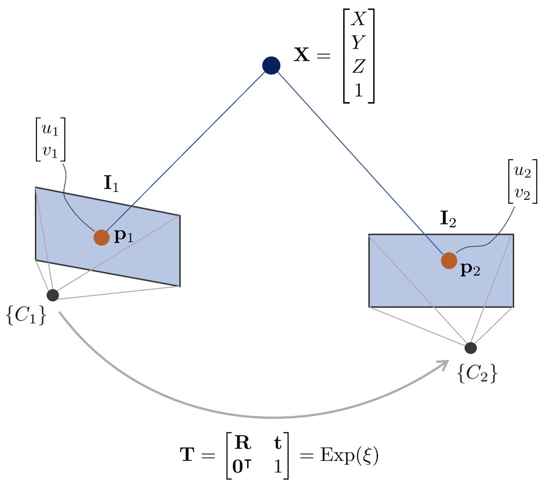
위 그림에서 3차원 점 $\mathbf{X}$의 월드 좌표는 $[X,Y,Z,1{]}^{⊺}\in {\mathbb{P}}^3$이고 이에 대응하는 두 카메라 이미지 평면 상의 픽셀 좌표는 ${\mathbf{p}}_1,{\mathbf{p}}_2\in {\mathbb{P}}^2$이다. 이 때, 두 카메라 $\{C_1\},\{C_2\}$의 내부 파라미터 $\mathbf{K}$는 동일하다고 가정한다. 카메라 $\{C_1\}$을 원점($\mathbf{R}=\mathbf{I},\mathbf{t}=\mathbf{0}$)이라고 했을 때 픽셀 좌표 ${\mathbf{p}}_1,{\mathbf{p}}_2$를 3차원 점 $\mathbf{X}$을 통해 표현하면 아래와 같은 순서로 프로젝션된다.

$$\begin{array}{}\text{(68)}& \begin{array}{r}\mathbf{p}=\pi (\mathbf{T},\mathbf{X})\end{array}\end{array}$$ 

$$\begin{array}{}\text{(69)}& \begin{array}{rl}{\mathbf{p}}_1=\left(\begin{array}{c}{u}_1\\ v_1\end{array}\right)& =\pi (\mathbf{I},\mathbf{X})={\pi }_k({\pi }_h(\mathbf{X}))\\ {\mathbf{p}}_2=\left(\begin{array}{c}{u}_2\\ v_2\end{array}\right)& =\pi (\mathbf{T},\mathbf{X})={\pi }_k({\pi }_h(\mathbf{TX}))\end{array}\end{array}$$ 

 

direct method의 특징 중 하나는 feature-based와 달리 어떤 ${\mathbf{p}}_2$가 ${\mathbf{p}}_1$과 매칭하는지 알 수 있는 방법이 없다. 따라서 현재 포즈 추정치를 기반으로 ${\mathbf{p}}_2$의 위치를 찾는다. 즉, 카메라의 포즈를 최적화하여 ${\mathbf{p}}_2$와 ${\mathbf{p}}_1$을 유사하게 만드는데 이 때 photometric 에러를 최소화하여 문제를 해결한다. photometric 에러는 다음과 같다.

$$\begin{array}{}\text{(70)}& \boxed{{\displaystyle \begin{array}{rl}\mathbf{e}(\mathbf{T})& ={\mathbf{I}}_1({\mathbf{p}}_1)-{\mathbf{I}}_2({\mathbf{p}}_2)\\ & ={\mathbf{I}}_1({\pi }_k({\pi }_h(\mathbf{X})))-{\mathbf{I}}_2({\pi }_k({\pi }_h(\mathbf{TX})))\end{array}}}\end{array}$$

 

photometric 에러는 grayscale 불변성 가정에 기반하며 스칼라 값을 가진다. photometric 에러를 통해 non-linear least squares를 풀기 위해 다음과 같은 에러 함수 $\mathbf{E}(\mathbf{T})$를 정의할 수 있다.

$$\begin{array}{}\text{(71)}& \begin{array}{rl}\mathbf{E}(\mathbf{T})& =\sum _{i\in \mathcal{P}}{\Vert {\mathbf{e}}_i(\mathbf{T})\Vert }^2\end{array}\end{array}$$
$$\begin{array}{}\text{(72)}& \begin{array}{rl}{\mathbf{T}}^{\ast }& =\arg \underset{{\mathbf{T}}^{\ast }}{min}\mathbf{E}(\mathbf{T})\\ & =\arg \underset{{\mathbf{T}}^{\ast }}{min}\sum _{i\in \mathcal{P}}{\Vert {\mathbf{e}}_i(\mathbf{T})\Vert }^2\\ & =\arg \underset{{\mathbf{T}}^{\ast }}{min}\sum _{i\in \mathcal{P}}{\mathbf{e}}_i(\mathbf{T}{)}^{⊺}{\mathbf{e}}_i(\mathbf{T})\\ & =\arg \underset{{\mathbf{T}}^{\ast }}{min}\sum _{i\in \mathcal{P}}({\mathbf{I}}_1({\mathbf{p}}_1^i)-{\mathbf{I}}_2({\mathbf{p}}_2^i){)}^{⊺}({\mathbf{I}}_1({\mathbf{p}}_1^i)-{\mathbf{I}}_2({\mathbf{p}}_2^i))\end{array}\end{array}$$

 

$\mathbf{E}({\mathbf{T}}^{\ast })$를 만족하는 ${\Vert \mathbf{e}({\mathbf{T}}^{\ast })\Vert }^2$를 non-linear least squares를 통해 반복적으로 계산할 수 있다. 작은 증분량 $\mathrm{\Delta }\mathbf{T}$를 반복적으로 $\mathbf{T}$에 업데이트함으로써 최적의 상태를 찾는다. 
$$\begin{array}{}\text{(73)}& \begin{array}{rl}\arg \underset{{\mathbf{T}}^{\ast }}{min}\mathbf{E}(\mathbf{T}+\mathrm{\Delta }\mathbf{T})& =\arg \underset{{\mathbf{T}}^{\ast }}{min}\sum _{i\in \mathcal{P}}{\Vert {\mathbf{e}}_i(\mathbf{T}+\mathrm{\Delta }\mathbf{T})\Vert }^2\end{array}\end{array}$$

 

엄밀하게 말하면 상태 증분량 $\mathrm{\Delta }\mathbf{T}$은 SE(3) 변환행렬이므로 $\oplus$ 연산자를 통해 기존 상태 $\mathbf{T}$에 더해지는게 맞지만 표현의 편의를 위해 $+$ 연산자를 사용하였다. 

$$\begin{array}{}\text{(74)}& \begin{array}{r}\mathbf{T}\oplus \mathrm{\Delta }\mathbf{T}\to \mathbf{T}+\mathrm{\Delta }\mathbf{T}\end{array}\end{array}$$

이는 1차 테일러 근사를 통해 다음과 같이 표현이 가능하다.
$$\begin{array}{}\text{(75)}& \begin{array}{rl}\mathbf{e}(\mathbf{T}+\mathrm{\Delta }\mathbf{T})& \approx {\mathbf{e}}_i(\mathbf{T})+\mathbf{J}\mathrm{\Delta }\mathbf{T}\\ & ={\mathbf{e}}_i(\mathbf{T})+\frac{\partial \mathbf{e}}{\partial \mathbf{T}}\mathrm{\Delta }\mathbf{T}\end{array}\end{array}$$

 

$$\begin{array}{}\text{(76)}& \begin{array}{rl}\arg \underset{{\mathbf{T}}^{\ast }}{min}\mathbf{E}(\mathbf{T}+\mathrm{\Delta }\mathbf{T})& =\arg \underset{{\mathbf{T}}^{\ast }}{min}\sum _{i\in \mathcal{P}}{\Vert {\mathbf{e}}_i(\mathbf{T})+\mathbf{J}\mathrm{\Delta }\mathbf{T}\Vert }^2\end{array}\end{array}$$

 

이를 미분하여 최적의 증분량 $\mathrm{\Delta }{\mathbf{T}}^{\ast }$ 값을 구하면 다음과 같다. 자세한 유도 과정은 본 섹션에서는 생략한다. 유도 과정에 대해 자세히 알고 싶으면 이전 섹션을 참조하면 된다.
$$\begin{array}{}\text{(77)}& \begin{array}{rl}& {\mathbf{J}}^{⊺}\mathbf{J}\mathrm{\Delta }{\mathbf{T}}^{\ast }=-{\mathbf{J}}^{⊺}\mathbf{e}\\ & \mathbf{H}\mathrm{\Delta }{\mathbf{T}}^{\ast }=-\mathbf{b}\end{array}\end{array}$$

위 식은 선형시스템 $\mathbf{Ax}=\mathbf{b}$ 형태이므로 schur complement, cholesky decomposition과 같은 다양한 선형대수학 테크닉을 사용하여 $\mathrm{\Delta }{\mathbf{T}}^{\ast }$를 구할 수 있다. 이렇게 구한 최적의 증분량을 현재 상태에 더한다. 이 때, 기존 상태 $\mathbf{T}$의 오른쪽에 곱하느냐 왼쪽에 곱하느냐에 따라서 각각 로컬 좌표계에서 본 포즈를 업데이트할 것 인지(오른쪽) 전역 좌표계에서 본 포즈를 업데이트할 것 인지(왼쪽) 달라지게 된다. Photometric 에러는 전역 좌표계의 변환 행렬을 업데이트하므로 일반적으로 왼쪽 곱셈 방법을 사용한다.
$$\begin{array}{}\text{(78)}& \begin{array}{r}\mathbf{T}\leftarrow \mathbf{T}\oplus \mathrm{\Delta }{\mathbf{T}}^{\ast }\end{array}\end{array}$$

 

왼쪽 곱셈 $\oplus$ 연산의 정의는 다음과 같다.

$$\begin{array}{}\text{(79)}& \begin{array}{rl}\mathbf{T}\oplus \mathrm{\Delta }{\mathbf{T}}^{\ast }& =\mathrm{\Delta }{\mathbf{T}}^{\ast }\mathbf{T}\\ & =\text{Exp}(\mathrm{\Delta }{\xi }^{\ast })\mathbf{T}\cdots \text{ globally updated (left mult)}\end{array}\end{array}$$

 

4.1. Jacobian of the photometric error

($\text{77}$)를 수행하기 위해서는 photometric 에러에 대한 자코비안 $\mathbf{J}$을 구해야 한다. 이는 다음과 같이 나타낼 수 있다.

$$\begin{array}{}\text{(80)}& \begin{array}{rl}\mathbf{J}& =\frac{\partial \mathbf{e}}{\partial \mathbf{T}}\\ & =\frac{\partial \mathbf{e}}{\partial [\mathbf{R},\mathbf{t}]}\end{array}\end{array}$$

 

이를 자세히 풀어서 보면 다음과 같다.

$$\begin{array}{}\text{(81)}& \begin{array}{rl}\mathbf{J}=\frac{\partial \mathbf{e}}{\partial \mathbf{T}}& =\frac{\partial }{\partial \mathbf{T}}({\mathbf{I}}_1({\mathbf{p}}_1)-{\mathbf{I}}_2({\mathbf{p}}_2))\\ & =\frac{\partial }{\partial \mathbf{T}}({\mathbf{I}}_1({\pi }_k({\pi }_h(\mathbf{X})))-{\mathbf{I}}_2({\pi }_k({\pi }_h(\mathbf{TX}))))\\ & =\frac{\partial }{\partial \mathbf{T}}(-{\mathbf{I}}_2({\pi }_k({\pi }_h(\mathbf{TX}))))\\ & =\frac{\partial }{\partial \mathbf{T}}(-{\mathbf{I}}_2({\pi }_k({\pi }_h({\mathbf{X}}^{\prime }))))\end{array}\end{array}$$

 

 

Chain rule을 적용하여 위 식을 다시 표현하면 다음과 같다.

$$\begin{array}{}\text{(82)}& \begin{array}{rl}\frac{\partial \mathbf{e}}{\partial \xi }& =\frac{\partial \mathbf{I}}{\partial {\mathbf{p}}_2}\frac{\partial {\mathbf{p}}_2}{\partial {\tilde{\mathbf{p}}}_2}\frac{\partial {\tilde{\mathbf{p}}}_2}{\partial {\mathbf{X}}^{\prime }}\frac{\partial {\mathbf{X}}^{\prime }}{\partial \xi }\\ & ={\mathbb{R}}^{1\times 2}\cdot {\mathbb{R}}^{2\times 3}\cdot {\mathbb{R}}^{3\times 4}\cdot {\mathbb{R}}^{4\times 6}={\mathbb{R}}^{1\times 6}\end{array}\end{array}$$

 

 

이 때, 변환행렬 $\mathbf{T}$에 대한 자코비안 $\frac{\partial {\mathbf{X}}^{\prime }}{\partial \mathbf{T}}$을 구하는 것이 아닌 twist $\xi$에 대한 자코비안 $\frac{\partial {\mathbf{X}}^{\prime }}{\partial \xi }$을 구하는 이유는 다음 섹션에서 설명한다.  우선 $\frac{\partial \mathbf{I}}{\partial {\mathbf{p}}_2}$은 이미지의 기울기(gradient)를 의미한다. 

$$\begin{array}{}\text{(83)}& \boxed{{\displaystyle \begin{array}{rl}\frac{\partial \mathbf{I}}{\partial {\mathbf{p}}_2}& =\left[\begin{array}{cc}\frac{\partial \mathbf{I}}{\partial u}& \frac{\partial \mathbf{I}}{\partial v}\end{array}\right]\\ & =\left[\begin{array}{cc}\mathrm{\nabla }{\mathbf{I}}_u& \mathrm{\nabla }{\mathbf{I}}_v\end{array}\right]\end{array}}}\end{array}$$

 

렌즈에 의한 왜곡(distortion)은 일반적으로 계산의 복잡성으로 인해 자코비안 계산 시 고려하지 않는다. 또한 렌즈 왜곡 보정(undistortion)이 이미지 입력 과정에서 이미 수행되었다고 가정하면 이를 고려할 필요가 없어진다.

따라서 $\frac{\partial {\mathbf{p}}_2}{\partial {\tilde{\mathbf{p}}}_2}$은 다음과 같이 단순히 카메라 내부 행렬 $\mathbf{K}$를 곱하는 것으로 구할 수 있다. 아래 수식에서는 마지막 행 $[001]$을 생략한 $\tilde{\mathbf{K}}$가 사용되었다.
$$\begin{array}{}\text{(84)}& \boxed{{\displaystyle \begin{array}{rl}\frac{\partial {\mathbf{p}}_2}{\partial {\tilde{\mathbf{p}}}_2}& =\frac{\partial }{\partial {\tilde{\mathbf{p}}}_2}\tilde{\mathbf{K}}{\tilde{\mathbf{p}}}_2\\ & =\tilde{\mathbf{K}}\\ & =\left[\begin{array}{ccc}f& 0& c_x\\ 0& f& c_y\end{array}\right]\in {\mathbb{R}}^{2\times 3}\end{array}}}\end{array}$$

다음으로 $\frac{\partial {\tilde{\mathbf{p}}}_2}{\partial {\mathbf{X}}^{\prime }}$은 다음과 같다.
$$\begin{array}{}\text{(85)}& \boxed{{\displaystyle \begin{array}{rl}\frac{\partial {\tilde{\mathbf{p}}}_2}{\partial {\mathbf{X}}^{\prime }}& =\frac{\partial [{\tilde{u}}_2,{\tilde{v}}_2,1]}{\partial [X^{\prime },Y^{\prime },Z^{\prime },1]}\\ & =\left[\begin{array}{cccc}\frac{1}{Z^{\prime }}& 0& \frac{-X^{\prime }}{Z^{\prime 2}}& 0\\ 0& \frac{1}{Z^{\prime }}& \frac{-Y^{\prime }}{Z^{\prime 2}}& 0\\ 0& 0& 0& 0\end{array}\right]\in {\mathbb{R}}^{3\times 4}\end{array}}}\end{array}$$

 

4.1.1. Lie theory-based SE(3) optimization

마지막으로 $\frac{\partial {\mathbf{X}}^{\prime }}{\partial \mathbf{T}}=\frac{\partial {\mathbf{X}}^{\prime }}{\partial [\mathbf{R},\mathbf{t}]}$를 구해야 한다. 이 때, 위치에 관련된 항 $\mathbf{t}$는 3차원 벡터이고 해당 벡터의 크기가 3차원 위치를 표현하는 최소한의 자유도인 3 자유도와 동일하므로 최적화 업데이트를 수행할 때 별도의 제약조건이 존재하지 않는다. 반면에, 회전행렬 $\mathbf{R}$은 파라미터의 개수가 9개이고 이는 3차원 회전을 표현하는 최소 자유도인 3 자유도보다 많으므로 다양한 제약조건이 존재한다. 이를 over-parameterized 되었다고 한다. over-parameterized 표현법의 단점은 다음과 같다.

• 중복되는 파라미터를 계산해야 하기 때문에 최적화 수행 시 연산량이 증가한다.
• 추가적인 자유도로 인해 수치적인 불안정성(numerical instability) 문제가 야기될 수 있다.
• 파라미터가 업데이트될 때마다 항상 제약조건을 만족하는 지 체크해줘야 한다.

 

따라서 제약조건으로 부터 자유로운 최소 파라미터(minimal parameter) 표현법인 lie theory 기반 최적화 방식을 일반적으로 사용한다. lie group SE(3) 기반 최적화 방법은 비선형의 회전행렬을 포함하는 $\mathrm{\Delta }{\mathbf{T}}^{\ast }$를 구하는 대신 회전 관련된 항은 $\mathbf{R}\to \mathbf{w}$으로 변경하고 위치 관련된 항은 $\mathbf{t}\to \mathbf{v}$로 변경하여 최적의 twist $\mathrm{\Delta }{\xi }^{\ast }$를 구한 후 lie algebra se(3) $[\mathrm{\Delta }\xi {]}_{\times }$를 exponential mapping을 통해 SE(3)에 업데이트 하는 방법을 말한다. 

$$\begin{array}{}\text{(86)}& \begin{array}{rl}\mathrm{\Delta }{\mathbf{T}}^{\ast }& \to \mathrm{\Delta }{\xi }^{\ast }\end{array}\end{array}$$

 

$\xi$에 대한 자코비안은 다음과 같다.

$$\begin{array}{}\text{(87)}& \begin{array}{rlrl}\mathbf{J}& =\frac{\partial \mathbf{e}}{\partial [\mathbf{R},\mathbf{t}]}& & \to \frac{\partial \mathbf{e}}{\partial [\mathbf{w},\mathbf{v}]}\\ & & & \to \frac{\partial \mathbf{e}}{\partial \xi }\end{array}\end{array}$$

 

이를 통해 기존의 식은 다음과 같이 변경된다.

$$\begin{array}{}\text{(88)}& \begin{array}{rl}\mathbf{e}(\mathbf{T})& \to \mathbf{e}(\xi )\\ \mathbf{E}(\mathbf{T})& \to \mathbf{E}(\xi )\\ \mathbf{e}(\mathbf{T})+{\mathbf{J}}^{\prime }\mathrm{\Delta }\mathbf{T}& \to \mathbf{e}(\xi )+\mathbf{J}\mathrm{\Delta }\xi \\ \mathbf{H}\mathrm{\Delta }{\mathbf{T}}^{\ast }=-\mathbf{b}& \to \mathbf{H}\mathrm{\Delta }{\xi }^{\ast }=-\mathbf{b}\\ \mathbf{T}\leftarrow \mathrm{\Delta }{\mathbf{T}}^{\ast }\mathbf{T}& \to \mathbf{T}\leftarrow \text{Exp}(\mathrm{\Delta }{\xi }^{\ast })\mathbf{T}\end{array}\end{array}$$

- ${\mathbf{J}}^{\prime }=\frac{\partial \mathbf{e}}{\partial \mathbf{T}}$

- $\mathbf{J}=\frac{\partial \mathbf{e}}{\partial \xi }$

 

$\text{Exp}(\xi )\in \text{SE}(3)$는 twist $\xi$를 exponential mapping하여 3차원 포즈로 변환하는 연산을 말한다. exponential mapping에 대한 자세한 내용은 해당 링크를 참조하면 된다.
$$\begin{array}{}\text{(89)}& \begin{array}{r}\text{Exp}(\mathrm{\Delta }\xi )=\mathrm{\Delta }\mathbf{T}\end{array}\end{array}$$

 

 

지금까지 자코비안들은 계산하기 용이했던 반면에 $\frac{\partial {\mathbf{X}}^{\prime }}{\partial \xi }$은 파라미터 $\xi$가 ${\mathbf{X}}^{\prime }$에서 바로 보이지 않으므로 ${\mathbf{X}}^{\prime }$를 lie algebra와 관련된 항으로 변경해야 한다. 

$$\begin{array}{}\text{(90)}& \begin{array}{r}{\mathbf{X}}^{\prime }\to \mathbf{TX}\to \text{Exp}(\xi )\mathbf{X}\end{array}\end{array}$$

 

이 때, 작은 lie algebra 증분량 $\mathrm{\Delta }\xi$를 기존 $\text{Exp}(\xi )$에 업데이트하는 방식에 따라 두 가지 방법으로 나뉘게 된다. 우선 [1] 기본적인 lie algebra를 사용한 업데이트 방법이 있다. 다음으로 [2] 섭동(perturbation) 모델을 활용한 업데이트 방법이 있다. 

$$\begin{array}{}\text{(91)}& \begin{array}{rl}\text{Exp}(\xi )& \leftarrow \text{Exp}(\xi +\mathrm{\Delta }\xi )\cdots \text{[1]}\\ \text{Exp}(\xi )& \leftarrow \text{Exp}(\mathrm{\Delta }\xi )\text{Exp}(\xi )\cdots \text{[2]}\end{array}\end{array}$$

 

위 두 방법 중 $[1]$ 방법은 기존 $\xi$에 미세 증분량 $\mathrm{\Delta }\xi$를 더한 후 exponential mapping을 수행하여 자코비안을 구하는 방법이며 $[2]$ 방법은 기존 $\xi$ 왼쪽에 섭동(perturbation) 모델 $\text{Exp}(\mathrm{\Delta }\xi )$을 곱함으로써 기존 상태를 업데이트하는 방법이다. 

 

두 방법 사이에는 다음과 같은 변환이 존재하며 이를 BCH 근사라고 한다. 자세한 내용은 Lie theory 개념 정리 포스팅을 참조하면 된다.
$$\begin{array}{}\text{(92)}& \begin{array}{rl}\text{Exp}(\mathrm{\Delta }\xi )\text{Exp}(\xi )& =\text{Exp}(\xi +{\mathcal{J}}_l^{-1}\mathrm{\Delta }\xi )\\ \text{Exp}(\xi +\mathrm{\Delta }\xi )& =\text{Exp}({\mathcal{J}}_l\mathrm{\Delta }\xi )\text{Exp}(\xi )\end{array}\end{array}$$

 

$[1]$ 방법을 사용하여 $\frac{\partial {\mathbf{X}}^{\prime }}{\partial \xi }$에 대한 자코비안을 계산하면 다음과 같다.
$$\begin{array}{}\text{(93)}& \boxed{{\displaystyle \begin{array}{rl}\frac{\partial {\mathbf{X}}^{\prime }}{\partial \mathrm{\Delta }\xi }& =\underset{\mathrm{\Delta }\xi \to 0}{lim}\frac{\text{Exp}(\xi +\mathrm{\Delta }\xi )-\text{Exp}(\xi )}{\mathrm{\Delta }\xi }\\ & =\underset{\mathrm{\Delta }\xi \to 0}{lim}\frac{\text{Exp}({\mathcal{J}}_l\mathrm{\Delta }\xi )\text{Exp}(\xi )-\text{Exp}(\xi )}{\mathrm{\Delta }\xi }\\ & \approx \underset{\mathrm{\Delta }\xi \to 0}{lim}\frac{(\mathbf{I}+[{\mathcal{J}}_l\mathrm{\Delta }\xi {]}_{\times })\text{Exp}(\xi )-\text{Exp}(\xi )}{\mathrm{\Delta }\xi }\\ & =\underset{\mathrm{\Delta }\xi \to 0}{lim}\frac{[{\mathcal{J}}_l\mathrm{\Delta }\xi {]}_{\times }{\mathbf{X}}^{\prime }}{\mathrm{\Delta }\xi }\\ & =\underset{\mathrm{\Delta }\xi \to 0}{lim}\frac{[\left[\begin{array}{cc}{\mathbf{J}}_l& {\mathbf{Q}}_l\\ \mathbf{0}& {\mathbf{J}}_l\end{array}\right]\left[\begin{array}{c}\mathrm{\Delta }\omega \\ \mathrm{\Delta }\mathbf{v}\end{array}\right]{]}_{\times }\left[\begin{array}{c}{\tilde{\mathbf{X}}}^{\prime }\\ 1\end{array}\right]}{\mathrm{\Delta }\xi }\\ & =\underset{\mathrm{\Delta }\xi \to 0}{lim}\frac{[\left[\begin{array}{c}{\mathbf{J}}_l\mathrm{\Delta }\omega +{\mathbf{Q}}_l\mathrm{\Delta }\mathbf{v}\\ {\mathbf{J}}_l\mathrm{\Delta }\mathbf{v}\end{array}\right]{]}_{\times }\left[\begin{array}{c}{\tilde{\mathbf{X}}}^{\prime }\\ 1\end{array}\right]}{\mathrm{\Delta }\xi }\\ & =\underset{\mathrm{\Delta }\xi \to 0}{lim}\frac{\left[\begin{array}{cc}[{\mathbf{J}}_l\mathrm{\Delta }\mathbf{w}+{\mathbf{Q}}_l\mathrm{\Delta }\mathbf{v}{]}_{\times }& {\mathbf{J}}_l\mathrm{\Delta }\mathbf{v}\\ {\mathbf{0}}^{⊺}& 0\end{array}\right]\left[\begin{array}{c}{\tilde{\mathbf{X}}}^{\prime }\\ 1\end{array}\right]}{\mathrm{\Delta }\xi }\\ & =\underset{\mathrm{\Delta }\xi \to 0}{lim}\frac{\left[\begin{array}{c}[{\mathbf{J}}_l\mathrm{\Delta }\mathbf{w}+{\mathbf{Q}}_l\mathrm{\Delta }\mathbf{v}{]}_{\times }{\tilde{\mathbf{X}}}^{\prime }+{\mathbf{J}}_l\mathrm{\Delta }\mathbf{v}\\ {\mathbf{0}}^{⊺}\end{array}\right]}{[\mathrm{\Delta }\mathbf{w},\mathrm{\Delta }\mathbf{v}{]}^{⊺}}\\ & =\underset{\mathrm{\Delta }\xi \to 0}{lim}\frac{\left[\begin{array}{c}-[{\tilde{\mathbf{X}}}^{\prime }{]}_{\times }({\mathbf{J}}_l\mathrm{\Delta }\mathbf{w}+{\mathbf{Q}}_l\mathrm{\Delta }\mathbf{v})+{\mathbf{J}}_l\mathrm{\Delta }\mathbf{v}\\ {\mathbf{0}}^{⊺}\end{array}\right]}{[\mathrm{\Delta }\mathbf{w},\mathrm{\Delta }\mathbf{v}{]}^{⊺}}\\ & =\left[\begin{array}{cc}-[{\tilde{\mathbf{X}}}^{\prime }{]}_{\times }{\mathbf{J}}_l& -[{\tilde{\mathbf{X}}}^{\prime }{]}_{\times }{\mathbf{Q}}_l+{\mathbf{J}}_l\\ {\mathbf{0}}^{⊺}& {\mathbf{0}}^{⊺}\end{array}\right]\in {\mathbb{R}}^{4\times 6}\end{array}}}\end{array}$$
- ${\mathcal{J}}_l=\left[\begin{array}{cc}{\mathbf{J}}_l& {\mathbf{Q}}_l\\ \mathbf{0}& {\mathbf{J}}_l\end{array}\right]$:  Lie theory 개념 정리 포스트 참조   

위 식에서 보다시피 $[1]$ 방법을 사용하면 매우 복잡한 식이 유도되기 때문에 해당 방법은 잘 사용되지 않고 $[2]$의 섭동 모델을 주로 사용한다. 따라서 $\frac{\partial {\mathbf{X}}^{\prime }}{\partial \xi }$은 다음과 같이 변형된다.
$$\begin{array}{}\text{(94)}& \begin{array}{rl}\frac{\partial {\mathbf{X}}^{\prime }}{\partial \xi }& \to \frac{\partial {\mathbf{X}}^{\prime }}{\partial \mathrm{\Delta }\xi }\end{array}\end{array}$$

 

$\frac{\partial {\mathbf{X}}^{\prime }}{\partial \mathrm{\Delta }\xi }$에 대한 자코비안은 다음과 같이 계산할 수 있다.

$$\begin{array}{}\text{(95)}& \boxed{{\displaystyle \begin{array}{rl}\frac{\partial {\mathbf{X}}^{\prime }}{\partial \mathrm{\Delta }\xi }& =\underset{\mathrm{\Delta }\xi \to 0}{lim}\frac{\text{Exp}(\mathrm{\Delta }\xi ){\mathbf{X}}^{\prime }-{\mathbf{X}}^{\prime }}{\mathrm{\Delta }\xi }\\ & \approx \underset{\mathrm{\Delta }\xi \to 0}{lim}\frac{(\mathbf{I}+[\mathrm{\Delta }\xi {]}_{\times }){\mathbf{X}}^{\prime }-{\mathbf{X}}^{\prime }}{\mathrm{\Delta }\xi }\\ & =\underset{\mathrm{\Delta }\xi \to 0}{lim}\frac{[\mathrm{\Delta }\xi {]}_{\times }{\mathbf{X}}^{\prime }}{\mathrm{\Delta }\xi }\\ & =\underset{\mathrm{\Delta }\xi \to 0}{lim}\frac{\left[\begin{array}{cc}[\mathrm{\Delta }\mathbf{w}{]}_{\times }& \mathrm{\Delta }\mathbf{v}\\ {\mathbf{0}}^{⊺}& 0\end{array}\right]\left[\begin{array}{c}{\tilde{\mathbf{X}}}^{\prime }\\ 1\end{array}\right]}{\mathrm{\Delta }\xi }\\ & =\underset{\mathrm{\Delta }\xi \to 0}{lim}\frac{\left[\begin{array}{c}-[{\tilde{\mathbf{X}}}^{\prime }{]}_{\times }\mathrm{\Delta }\mathbf{w}+\mathrm{\Delta }\mathbf{v}\\ {\mathbf{0}}^{⊺}\end{array}\right]}{[\mathrm{\Delta }\mathbf{w},\mathrm{\Delta }\mathbf{v}{]}^{⊺}}\\ & =\left[\begin{array}{cc}-[{\tilde{\mathbf{X}}}^{\prime }{]}_{\times }& \mathbf{I}\\ {\mathbf{0}}^{⊺}& {\mathbf{0}}^{⊺}\end{array}\right]\in {\mathbb{R}}^{4\times 6}\end{array}}}\end{array}$$

 

따라서 $[2]$ 섭동 모델을 사용하는 경우 3차원 공간 상의 점 ${\mathbf{X}}^{\prime }$의 반대칭 행렬을 사용하여 간단하게 자코비안을 구할 수 있는 이점이 있다. photometric 에러 최적화의 경우 대부분 순차적으로 들어오는 이미지들의 밝기 변화에 대한 에러를 최적화하므로 카메라 포즈 변화가 크지 않고 따라서 $\mathrm{\Delta }\xi$의 크기 또한 크지 않으므로 일반적으로 위의 자코비안을 주로 사용한다. $[2]$ 섭동 모델을 사용하므로 작은 증분량 $\mathrm{\Delta }{\xi }^{\ast }$는 ($\text{79}$)와 같이 업데이트된다.

$$\begin{array}{}\text{(96)}& \begin{array}{r}\mathbf{T}\leftarrow \mathrm{\Delta }{\mathbf{T}}^{\ast }\mathbf{T}=\text{Exp}(\mathrm{\Delta }{\xi }^{\ast })\mathbf{T}\end{array}\end{array}$$

 

위 식에서 두 번째 행은 작은 twist 증분량 $\text{Exp}(\mathrm{\Delta }\xi )$에 대해 1차 테일러 근사가 적용된 형태이다. 두 번째 행의 근사를 이해하기 위해 임의의 twist $\xi =[\mathbf{w},\mathbf{v}{]}^{⊺}$가 주어졌을 때 변환행렬 $\mathbf{T}$를 exponential mapping 형태로 전개하면 다음과 같이 나타낼 수 있다. $$\begin{array}{}\text{(97)}& \begin{array}{rl}\mathbf{T}& =\text{Exp}(\xi )\\ & =\exp ([\xi {]}_{\times })\\ & =\mathbf{I}+\left[\begin{array}{cc}[\mathbf{w}{]}_{\times }& \mathbf{v}\\ {\mathbf{0}}^{⊺}& 0\end{array}\right]+\frac{1}{2!}\left[\begin{array}{cc}[\mathbf{w}{]}_{\times }^2& [\mathbf{w}{]}_{\times }\mathbf{v}\\ {\mathbf{0}}^{⊺}& 0\end{array}\right]+\frac{1}{3!}\left[\begin{array}{cc}[\mathbf{w}{]}_{\times }^3& [\mathbf{w}{]}_{\times }^2\mathbf{v}\\ {\mathbf{0}}^{⊺}& 0\end{array}\right]+\cdots \\ & =\mathbf{I}+[\xi {]}_{\times }+\frac{1}{2!}[\xi {]}_{\times }^2+\frac{1}{3!}[\xi {]}_{\times }^3+\cdots \end{array}\end{array}$$

작은 크기의 twist 증분량 $\mathrm{\Delta }\xi$에 대해서는 2차 이상의 고차항을 무시하여 다음과 같이 근사적으로 나타낼 수 있다. $$\begin{array}{}\text{(98)}& \begin{array}{r}\text{Exp}(\mathrm{\Delta }\xi )\approx \mathbf{I}+[\mathrm{\Delta }\xi {]}_{\times }\end{array}\end{array}$$

 

최종적인 포즈에 대한 자코비안 $\mathbf{J}$은 다음과 같다. 

$$\begin{array}{}\text{(99)}& \boxed{{\displaystyle \begin{array}{rl}\mathbf{J}=\frac{\partial \mathbf{e}}{\partial \mathrm{\Delta }\xi }& =\frac{\partial \mathbf{I}}{\partial {\mathbf{p}}_2}\frac{\partial {\mathbf{p}}_2}{\partial {\tilde{\mathbf{p}}}_2}\frac{\partial {\tilde{\mathbf{p}}}_2}{\partial {\mathbf{X}}^{\prime }}\frac{\partial {\mathbf{X}}^{\prime }}{\partial \mathrm{\Delta }\xi }\\ & =\left[\begin{array}{cc}\mathrm{\nabla }{\mathbf{I}}_u& \mathrm{\nabla }{\mathbf{I}}_v\end{array}\right]\left[\begin{array}{ccc}f& 0& c_x\\ 0& f& c_y\end{array}\right]\left[\begin{array}{cccc}\frac{1}{Z^{\prime }}& 0& \frac{-X^{\prime }}{Z^{\prime 2}}& 0\\ 0& \frac{1}{Z^{\prime }}& \frac{-Y^{\prime }}{Z^{\prime 2}}& 0\\ 0& 0& 0& 0\end{array}\right]\left[\begin{array}{cc}-[{\tilde{\mathbf{X}}}^{\prime }{]}_{\times }& \mathbf{I}\\ {\mathbf{0}}^{⊺}& {\mathbf{0}}^{⊺}\end{array}\right]\\ & =\left[\begin{array}{cc}\mathrm{\nabla }{\mathbf{I}}_u& \mathrm{\nabla }{\mathbf{I}}_v\end{array}\right]\left[\begin{array}{cccc}\frac{f}{Z^{\prime }}& 0& -\frac{fX}{Z^{\prime 2}}& 0\\ 0& \frac{f}{Z^{\prime }}& -\frac{fY}{Z^{\prime 2}}& 0\end{array}\right]\left[\begin{array}{cccccc}0& Z^{\prime }& -Y^{\prime }& 1& 0& 0\\ -Z^{\prime }& 0& X^{\prime }& 0& 1& 0\\ Y^{\prime }& -X^{\prime }& 0& 0& 0& 1\\ 0& 0& 0& 0& 0& 0\end{array}\right]\\ & =\left[\begin{array}{cc}\mathrm{\nabla }{\mathbf{I}}_u& \mathrm{\nabla }{\mathbf{I}}_v\end{array}\right]\left[\begin{array}{cccccc}-\frac{f{X}^{\prime }{Y}^{\prime }}{Z^{\prime 2}}& \frac{f(1+X^{\prime 2})}{Z^{\prime 2}}& -\frac{f{Y}^{\prime }}{Z^{\prime }}& \frac{f}{Z^{\prime }}& 0& -\frac{f{X}^{\prime }}{Z^{\prime 2}}\\ -\frac{f(1+Y^{\prime 2})}{Z^{\prime 2}}& \frac{f{X}^{\prime }{Y}^{\prime }}{Z^{\prime 2}}& \frac{f{X}^{\prime }}{Z^{\prime }}& 0& \frac{f}{Z^{\prime }}& -\frac{f{Y}^{\prime }}{Z^{\prime 2}}\end{array}\right]\in {\mathbb{R}}^{1\times 6}\end{array}}}\end{array}$$

이 때, $\frac{\partial {\mathbf{X}}^{\prime }}{\partial \mathrm{\Delta }\xi }$의 마지막 행은 항상 0이므로 이를 생략하고 계산하기도 한다.

 

4.2. Code implementations

• Visual SLAM 입문 챕터8 코드: direct_sparse.cpp#L111
• DSO 코드: CoarseInitializer.cpp#L430
• DSO 코드2: CoarseTracker.cpp#L320

 

 

5. Relative pose error

Relative pose 에러는 주로 pose graph optimization(PGO)에서 사용하는 에러이다. PGO에 대한 자세한 내용은 [SLAM] Pose Graph Optimization 개념 설명 및 예제 코드 분석 포스트를 참조하면 된다.

 

NOMENCLATURE of relative pose error

• $\text{(Node) }{\mathbf{x}}_i=\left[\begin{array}{cc}{\mathbf{R}}_i& {\mathbf{t}}_i\\ {\mathbf{0}}^{⊺}& 1\end{array}\right]\in {\mathbb{R}}^{4\times 4}$
• $\text{(Edge) }{\mathbf{z}}_{ij}=\left[\begin{array}{cc}{\mathbf{R}}_{ij}& {\mathbf{t}}_{ij}\\ {\mathbf{0}}^{⊺}& 1\end{array}\right]\in {\mathbb{R}}^{4\times 4}$
• ${\hat{\mathbf{z}}}_{ij}={\mathbf{x}}_i^{-1}{\mathbf{x}}_j$ : 예측값
• ${\mathbf{z}}_{ij}$ : 관측값 (virtual measurement)
• $\mathbf{x}=[{\mathbf{x}}_1,\cdots ,{\mathbf{x}}_n]$: pose graph의 모든 포즈 노드
• ${\mathbf{e}}_{ij}({\mathbf{x}}_i,{\mathbf{x}}_j)\leftrightarrow {\mathbf{e}}_{ij}$: 표현의 편의를 위해 생략하여 표기하기도 한다.
• $\mathbf{J}=\frac{\partial \mathbf{e}}{\partial \mathbf{x}}$
• $\oplus$ : 두 SE(3) 군을 결합(composition)하는 연산자
• $\text{Log}(\cdot )$: SE(3)를 twist $\xi \in {\mathbb{R}}^6$로 변환하는 연산자. Logarithm mapping에 대한 자세한 내용은 해당 포스트를 참조하면 된다.
• $\text{Exp}(\xi )=\exp ([\xi {]}_{\times })$

 

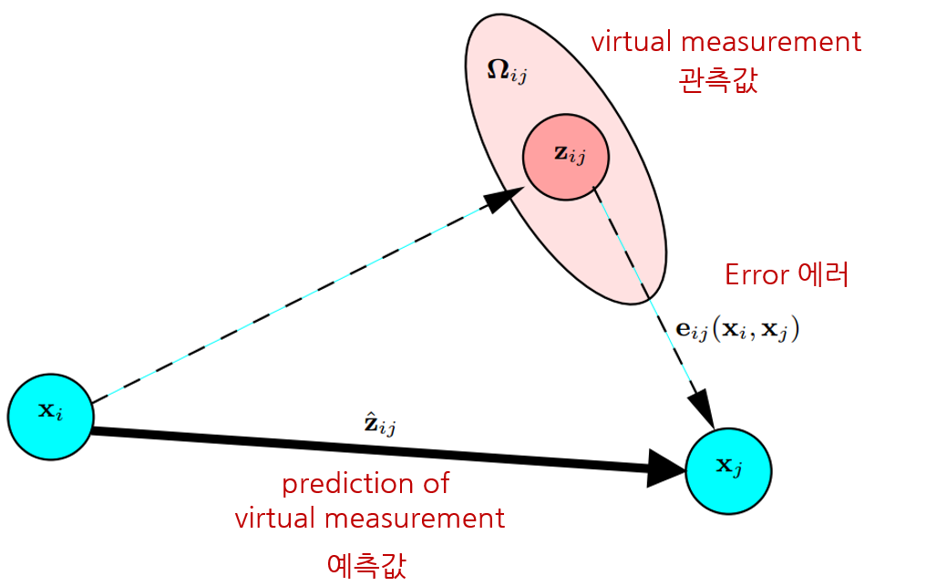
Pose graph 상에서 두 노드 ${\mathbf{x}}_i,{\mathbf{x}}_j$가 주어졌을 때 센서 데이터에 의해 새롭게 계산한 상대포즈(관측값) ${\mathbf{z}}_{ij}$와 기존의 알고 있는 상대포즈(예측값) ${\hat{\mathbf{z}}}_{ij}$의 차이를 relative pose 에러로 정의한다. (Freiburg univ. Robot Mapping Course 그림 참조).

$$\begin{array}{}\text{(100)}& \begin{array}{r}{\mathbf{e}}_{ij}({\mathbf{x}}_i,{\mathbf{x}}_j)={\mathbf{z}}_{ij}^{-1}{\hat{\mathbf{z}}}_{ij}={\mathbf{z}}_{ij}^{-1}{\mathbf{x}}_i^{-1}{\mathbf{x}}_j\end{array}\end{array}$$

 

relative pose 에러를 최적화하는 과정을 pose graph optimization(PGO)라고 하며 graph-based SLAM의 back-end 알고리즘으로도 불린다. Front-end의 visual odometry(VO) 또는 lidar odometry(LO)에 의해 순차적으로 계산되는 노드 ${\mathbf{x}}_i,{\mathbf{x}}_{i+1},\cdots$는 관측값과 예측값이 동일하기 때문에 PGO가 수행되지 않지만 loop closing이 발생하여 비순차적인 두 노드 ${\mathbf{x}}_i,{\mathbf{x}}_j$ 사이에 엣지가 연결되면 관측값과 예측값의 차이가 발생하기 때문에 PGO가 수행된다. 

 

즉, PGO는 일반적으로 loop closing과 같은 특수한 상황이 발생할 때 수행된다. 로봇이 이동하면서 같은 장소를 재방문하는 경우 loop detection 알고리즘이 동작하여 루프를 판별한다. 이 때 루프가 탐지되면 기존 노드 ${\mathbf{x}}_i$와 재방문하여 생성된 노드 ${\mathbf{x}}_j$가 loop edge로 연결되고 여러 매칭 알고리즘 (GICP, NDT, etc...)에 의해 관측값을 생성한다. 이러한 관측값은 실제로 관측한 값이 아닌 매칭 알고리즘에 의해 생성된 가상의 관측값이므로 virtual measurement라고 불린다.

 

Pose graph 상의 모든 노드에 대한 relative pose 에러는 다음과 같이 정의할 수 있다.

$$\begin{array}{}\text{(101)}& \begin{array}{rl}\mathbf{E}(\mathbf{x})& =\sum _i\sum _j{\Vert {\mathbf{e}}_{ij}(\mathbf{x})\Vert }^2\end{array}\end{array}$$
$$\begin{array}{}\text{(102)}& \begin{array}{rl}{\mathbf{x}}^{\ast }& =\arg \underset{{\mathbf{x}}^{\ast }}{min}\mathbf{E}(\mathbf{x})\\ & =\arg \underset{{\mathbf{x}}^{\ast }}{min}\sum _i\sum _j{\Vert {\mathbf{e}}_{ij}(\mathbf{x})\Vert }^2\\ & =\arg \underset{{\mathbf{x}}^{\ast }}{min}\sum _i\sum _j{\mathbf{e}}_{ij}(\mathbf{x}{)}^{⊺}{\mathbf{e}}_{ij}(\mathbf{x})\end{array}\end{array}$$

 

$\mathbf{E}({\mathbf{x}}^{\ast })$를 만족하는 ${\Vert \mathbf{e}({\mathbf{x}}^{\ast })\Vert }^2$를 non-linear least squares를 통해 반복적으로 계산할 수 있다. 작은 증분량 $\mathrm{\Delta }\mathbf{x}$를 반복적으로 $\mathbf{x}$에 업데이트함으로써 최적의 상태를 찾는다. 
$$\begin{array}{}\text{(103)}& \begin{array}{rl}\arg \underset{{\mathbf{x}}^{\ast }}{min}\mathbf{E}(\mathbf{x}+\mathrm{\Delta }\mathbf{x})& =\arg \underset{{\mathbf{x}}^{\ast }}{min}\sum _i\sum _j{\Vert {\mathbf{e}}_{ij}({\mathbf{x}}_i+\mathrm{\Delta }{\mathbf{x}}_i,{\mathbf{x}}_j+\mathrm{\Delta }{\mathbf{x}}_j)\Vert }^2\end{array}\end{array}$$

엄밀하게 말하면 상태 증분량 $\mathrm{\Delta }\mathbf{x}$은 SE(3) 변환행렬이므로 $\oplus$ 연산자를 통해 기존 상태 $\mathbf{x}$에 더해지는게 맞지만 표현의 편의를 위해 $+$ 연산자를 사용하였다.

$$\begin{array}{}\text{(104)}& \begin{array}{r}{\mathbf{e}}_{ij}({\mathbf{x}}_i\oplus \mathrm{\Delta }{\mathbf{x}}_i,{\mathbf{x}}_j\oplus \mathrm{\Delta }{\mathbf{x}}_j)\to {\mathbf{e}}_{ij}({\mathbf{x}}_i+\mathrm{\Delta }{\mathbf{x}}_i,{\mathbf{x}}_j+\mathrm{\Delta }{\mathbf{x}}_j)\end{array}\end{array}$$

 

위 식은 테일러 1차 근사를 통해 다음과 같이 표현이 가능하다.
$$\begin{array}{}\text{(105)}& \begin{array}{rl}{\mathbf{e}}_{ij}({\mathbf{x}}_i+\mathrm{\Delta }{\mathbf{x}}_i,{\mathbf{x}}_j+\mathrm{\Delta }{\mathbf{x}}_j)& \approx {\mathbf{e}}_{ij}({\mathbf{x}}_i,{\mathbf{x}}_j)+{\mathbf{J}}_{ij}\left[\begin{array}{c}\mathrm{\Delta }{\mathbf{x}}_i\\ \mathrm{\Delta }{\mathbf{x}}_j\end{array}\right]\\ & ={\mathbf{e}}_{ij}({\mathbf{x}}_i,{\mathbf{x}}_j)+{\mathbf{J}}_i\mathrm{\Delta }{\mathbf{x}}_i+{\mathbf{J}}_j\mathrm{\Delta }{\mathbf{x}}_j\\ & ={\mathbf{e}}_{ij}({\mathbf{x}}_i,{\mathbf{x}}_j)+\frac{\partial {\mathbf{e}}_{ij}}{\partial {\mathbf{x}}_i}\mathrm{\Delta }{\mathbf{x}}_i++\frac{\partial {\mathbf{e}}_{ij}}{\partial {\mathbf{x}}_j}\mathrm{\Delta }{\mathbf{x}}_j\end{array}\end{array}$$

 

$$\begin{array}{}\text{(106)}& \begin{array}{rl}\arg \underset{{\mathbf{x}}^{\ast }}{min}\mathbf{E}(\mathbf{x}+\mathrm{\Delta }\mathbf{x})& \approx \arg \underset{{\mathbf{x}}^{\ast }}{min}\sum _i\sum _j{\Vert {\mathbf{e}}_{ij}({\mathbf{x}}_i,{\mathbf{x}}_j)+{\mathbf{J}}_{ij}\left[\begin{array}{c}\mathrm{\Delta }{\mathbf{x}}_i\\ \mathrm{\Delta }{\mathbf{x}}_j\end{array}\right]\Vert }^2\end{array}\end{array}$$

 

이를 미분하여 모든 노드에 대한 최적의 증분량 $\mathrm{\Delta }{\mathbf{x}}^{\ast }$ 값을 구하면 다음과 같다. 자세한 유도 과정은 본 섹션에서는 생략한다. 유도 과정에 대해 자세히 알고 싶으면 이전 섹션을 참조하면 된다.
$$\begin{array}{}\text{(107)}& \begin{array}{rl}& {\mathbf{J}}^{⊺}\mathbf{J}\mathrm{\Delta }{\mathbf{x}}^{\ast }=-{\mathbf{J}}^{⊺}\mathbf{e}\\ & \mathbf{H}\mathrm{\Delta }{\mathbf{x}}^{\ast }=-\mathbf{b}\end{array}\end{array}$$

 

위 식은 선형시스템 $\mathbf{Ax}=\mathbf{b}$ 형태이므로 schur complement, cholesky decomposition과 같은 다양한 선형대수학 테크닉을 사용하여 $\mathrm{\Delta }{\mathbf{x}}^{\ast }$를 구할 수 있다. 이렇게 구한 최적의 증분량을 현재 상태에 더한다. 이 때, 기존 상태 $\mathbf{x}$의 오른쪽에 곱하느냐 왼쪽에 곱하느냐에 따라서 각각 로컬 좌표계에서 본 포즈를 업데이트할 것 인지(오른쪽) 전역 좌표계에서 본 포즈를 업데이트할 것 인지(왼쪽) 달라지게 된다. relative pose 에러는 두 노드의 상대 포즈에 관련되어 있으므로 로컬 좌표계에서 업데이트하는 오른쪽 곱셈이 적용된다.
$$\begin{array}{}\text{(108)}& \begin{array}{r}\mathbf{x}\leftarrow \mathbf{x}\oplus \mathrm{\Delta }{\mathbf{x}}^{\ast }\end{array}\end{array}$$

 

오른쪽 곱셈 $\oplus$ 연산의 정의는 다음과 같다.

$$\begin{array}{}\text{(109)}& \begin{array}{rl}\mathbf{x}\oplus \mathrm{\Delta }{\mathbf{x}}^{\ast }& =\mathbf{x}\mathrm{\Delta }{\mathbf{x}}^{\ast }\\ & =\mathbf{x}\text{Exp}(\mathrm{\Delta }{\xi }^{\ast })\cdots \text{ locally updated (right mult)}\end{array}\end{array}$$

 

 

5.1. Jacobian of relative pose error

($\text{107}$)를 수행하기 위해서는 relative pose 에러에 대한 자코비안 $\mathbf{J}$을 구해야 한다. 비순차적인 두 노드 ${\mathbf{x}}_i,{\mathbf{x}}_j$가 주어졌을 때 이에 대한 자코비안 ${\mathbf{J}}_{ij}$ 다음과 같이 나타낼 수 있다.

$$\begin{array}{}\text{(110)}& \begin{array}{rl}{\mathbf{J}}_{ij}& =\frac{\partial {\mathbf{e}}_{ij}}{\partial {\mathbf{x}}_{ij}}\\ & =\frac{\partial {\mathbf{e}}_{ij}}{\partial [{\mathbf{x}}_i,{\mathbf{x}}_j]}\\ & =[{\mathbf{J}}_i,{\mathbf{J}}_j]\end{array}\end{array}$$

 

이를 자세히 풀어서 보면 다음과 같다.

$$\begin{array}{}\text{(111)}& \begin{array}{rl}{\mathbf{J}}_{ij}=\frac{\partial {\mathbf{e}}_{ij}}{\partial [{\mathbf{x}}_i,{\mathbf{x}}_j]}& =\frac{\partial }{\partial [{\mathbf{x}}_i,{\mathbf{x}}_j]}({\mathbf{z}}_{ij}^{-1}{\hat{\mathbf{z}}}_{ij})\\ & =\frac{\partial }{\partial [{\mathbf{R}}_i,{\mathbf{t}}_i,{\mathbf{R}}_j,{\mathbf{t}}_j]}({\mathbf{z}}_{ij}^{-1}{\hat{\mathbf{z}}}_{ij})\end{array}\end{array}$$

 

5.1.1. Lie theory-based SE(3) optimization

위 자코비안을 구할 때, 위치에 관련된 항 $\mathbf{t}$는 3차원 벡터이고 해당 벡터의 크기가 3차원 위치를 표현하는 최소한의 자유도인 3 자유도와 동일하므로 최적화 업데이트를 수행할 때 별도의 제약조건이 존재하지 않는다. 반면에, 회전행렬 $\mathbf{R}$은 파라미터의 개수가 9개이고 이는 3차원 회전을 표현하는 최소 자유도인 3 자유도보다 많으므로 다양한 제약조건이 존재한다. 이를 over-parameterized 되었다고 한다. over-parameterized 표현법의 단점은 다음과 같다.

• 중복되는 파라미터를 계산해야 하기 때문에 최적화 수행 시 연산량이 증가한다.
• 추가적인 자유도로 인해 수치적인 불안정성(numerical instability) 문제가 야기될 수 있다.
• 파라미터가 업데이트될 때마다 항상 제약조건을 만족하는 지 체크해줘야 한다.

 

따라서 제약조건으로 부터 자유로운 최소 파라미터(minimal parameter) 표현법인 lie theory 기반 최적화 방식을 일반적으로 사용한다. lie group SE(3) 기반 최적화 방법은 비선형의 회전행렬을 포함하는 $\mathrm{\Delta }{\mathbf{T}}^{\ast }$를 구하는 대신 회전 관련된 항은 $\mathbf{R}\to \mathbf{w}$으로 변경하고 위치 관련된 항은 $\mathbf{t}\to \mathbf{v}$로 변경하여 최적의 twist $\mathrm{\Delta }{\xi }^{\ast }$를 구한 후 lie algebra se(3) $[\mathrm{\Delta }\xi {]}_{\times }$를 exponential mapping을 통해 SE(3)에 업데이트 하는 방법을 말한다.

$$\begin{array}{}\text{(112)}& \begin{array}{r}\left[\begin{array}{c}\mathrm{\Delta }{\mathbf{x}}_i^{\ast },\mathrm{\Delta }{\mathbf{x}}_j^{\ast }\end{array}\right]\to [\mathrm{\Delta }{\xi }_i^{\ast },\mathrm{\Delta }{\xi }_j^{\ast }]\end{array}\end{array}$$

 

$\xi$에 대한 자코비안은 다음과 같다.

$$\begin{array}{}\text{(113)}& \begin{array}{rlrl}{\mathbf{J}}_{ij}& =\frac{\partial {\mathbf{e}}_{ij}}{\partial [{\mathbf{x}}_i,{\mathbf{x}}_j]}& & \to \frac{\partial {\mathbf{e}}_{ij}}{\partial [{\xi }_i,{\xi }_j]}\end{array}\end{array}$$

 

이를 통해 기존의 식은 다음과 같이 변경된다.

$$\begin{array}{}\text{(114)}& \begin{array}{rl}{\mathbf{e}}_{ij}({\mathbf{x}}_i,{\mathbf{x}}_j)& \to {\mathbf{e}}_{ij}({\xi }_i,{\xi }_j)\\ \mathbf{E}(\mathbf{x})& \to \mathbf{E}(\xi )\\ {\mathbf{e}}_{ij}({\mathbf{x}}_i,{\mathbf{x}}_j)+{\mathbf{J}}_i^{\prime }\mathrm{\Delta }{\mathbf{x}}_i+{\mathbf{J}}_j^{\prime }\mathrm{\Delta }{\mathbf{x}}_j& \to {\mathbf{e}}_{ij}({\xi }_i,{\xi }_j)+{\mathbf{J}}_i\mathrm{\Delta }{\xi }_i+{\mathbf{J}}_j\mathrm{\Delta }{\xi }_j\\ \mathbf{H}\mathrm{\Delta }{\mathbf{x}}^{\ast }=-\mathbf{b}& \to \mathbf{H}\mathrm{\Delta }{\xi }^{\ast }=-\mathbf{b}\\ \mathbf{x}\leftarrow \mathrm{\Delta }{\mathbf{x}}^{\ast }\mathbf{x}& \to \mathbf{x}\leftarrow \text{Exp}(\mathrm{\Delta }{\xi }^{\ast })\mathbf{x}\end{array}\end{array}$$

- ${\mathbf{J}}_{ij}^{\prime }=\frac{\partial \mathbf{e}}{\partial [{\mathbf{x}}_i,{\mathbf{x}}_j]}$

- ${\mathbf{J}}_{ij}=\frac{\partial \mathbf{e}}{\partial [{\xi }_i,{\xi }_j]}$

 

$\text{Exp}(\xi )\in \text{SE}(3)$는 twist $\xi$를 exponential mapping하여 3차원 포즈로 변환하는 연산을 말한다. exponential mapping에 대한 자세한 내용은 해당 링크를 참조하면 된다. $$\begin{array}{}\text{(115)}& \begin{array}{r}\text{Exp}(\mathrm{\Delta }\xi )=\mathrm{\Delta }\mathbf{x}\end{array}\end{array}$$

 

$\frac{\partial }{\partial \xi }({\mathbf{z}}_{ij}^{-1}{\hat{\mathbf{z}}}_{ij})$은 파라미터 $\xi$가 ${\mathbf{z}}_{ij}^{-1}{\hat{\mathbf{z}}}_{ij}$에서 바로 보이지 않으므로 이를 lie algebra와 관련된 항으로 변경해야 한다. 

$$\begin{array}{}\text{(116)}& \begin{array}{rl}{\mathbf{z}}_{ij}^{-1}{\hat{\mathbf{z}}}_{ij}& \to \text{Log}({\mathbf{z}}_{ij}^{-1}{\hat{\mathbf{z}}}_{ij})\end{array}\end{array}$$

 

이 때, $\text{Log}(\cdot )$는 SE(3)에서 twist $\xi \in {\mathbb{R}}^6$로 변경하는 logarithm mapping을 의미한다.  Logarithm mapping에 대한 자세한 내용은 해당 포스트를 참조하면 된다. 따라서 SE(3) 버전 relative pose 에러 ${\mathbf{e}}_{ij}$는 다음과 같이 변경된다.
$$\begin{array}{}\text{(117)}& \boxed{{\displaystyle \begin{array}{rl}{\mathbf{e}}_{ij}({\mathbf{x}}_i,{\mathbf{x}}_j)={\mathbf{z}}_{ij}^{-1}{\hat{\mathbf{z}}}_{ij}\to {\mathbf{e}}_{ij}({\xi }_i,{\xi }_j)& =\text{Log}({\mathbf{z}}_{ij}^{-1}{\hat{\mathbf{z}}}_{ij})\end{array}}}\end{array}$$

 

이를 자세히 풀어쓰면 다음과 같다.

$$\begin{array}{}\text{(118)}& \begin{array}{rl}{\mathbf{e}}_{ij}({\xi }_i,{\xi }_j)& =\text{Log}({\mathbf{z}}_{ij}^{-1}{\hat{\mathbf{z}}}_{ij})\\ & =\text{Log}({\mathbf{z}}_{ij}^{-1}{\mathbf{x}}_i^{-1}{\mathbf{x}}_j)\\ & =\text{Log}(\text{Exp}(-{\xi }_{ij})\text{Exp}(-{\xi }_i)\text{Exp}({\xi }_j))\end{array}\end{array}$$

 

위 식을 보면 ${\mathbf{z}}_{ij}$ 안에 ${\xi }_i,{\xi }_j$ 파라미터가 exponential mapping으로 연결되어 있는 것을 알 수 있다. 위 식 두 번째 라인의 공식에 왼쪽 섭동(perturbation) 모델을 적용하여 증분량을 표현하면 다음과 같다.

$$\begin{array}{}\text{(119)}& \begin{array}{rl}{\mathbf{e}}_{ij}({\xi }_i+\mathrm{\Delta }{\xi }_i,{\xi }_j+\mathrm{\Delta }{\xi }_j)& =\text{Log}({\hat{\mathbf{z}}}_{ij}^{-1}{\mathbf{x}}_i^{-1}\text{Exp}(-\mathrm{\Delta }{\xi }_i)\text{Exp}(\mathrm{\Delta }{\xi }_j){\mathbf{x}}_j)\end{array}\end{array}$$

 

위 식에서 증분량 항을 왼쪽 또는 오른쪽으로 이동시켜야 $\mathbf{e}+\mathbf{J}\mathrm{\Delta }\xi$ 꼴로 항이 정리된다. 이를 수행하기 위해 아래와 같은 adjoint matrix of SE(3)의 성질을 이용해야 한다. Adjoint martix에 대한 자세한 내용은 해당 포스트를 참조하면 된다. $$\begin{array}{}\text{(120)}& \begin{array}{r}\text{Exp}({\text{Ad}}_{\mathbf{T}}\xi )=\mathbf{T}\text{Exp}(\xi ){\mathbf{T}}^{-1}\end{array}\end{array}$$

위 식을 $\mathbf{T}\to {\mathbf{T}}^{-1}$에 대한 식으로 변형하면 다음과 같다. $$\begin{array}{}\text{(121)}& \begin{array}{r}\text{Exp}({\text{Ad}}_{{\mathbf{T}}^{-1}}\xi )={\mathbf{T}}^{-1}\text{Exp}(\xi )\mathbf{T}\end{array}\end{array}$$

그리고 정리하면 다음과 같은 공식을 얻을 수 있다. $$\begin{array}{}\text{(122)}& \begin{array}{r}\text{Exp}(\xi )\mathbf{T}=\mathbf{T}\text{Exp}({\text{Ad}}_{{\mathbf{T}}^{-1}}\xi )\end{array}\end{array}$$

 

($\text{122}$)을 사용하면 ($\text{119}$)의 중간에 있는 $\text{Exp}(\cdot )\text{Exp}(\cdot )$ 항을 오른쪽 또는 왼쪽으로 이동시킬 수 있다. 본 포스트에서는 오른쪽으로 이동시키는 과정에 대해 설명한다. 이를 $\mathrm{\Delta }{\xi }_i,\mathrm{\Delta }{\xi }_j$ 별로 각각 전개하면 다음과 같다.

$$\begin{array}{}\text{(123)}& \begin{array}{rl}{\mathbf{e}}_{ij}({\xi }_i+\mathrm{\Delta }{\xi }_i,{\xi }_j)& =\text{Log}({\hat{\mathbf{z}}}_{ij}^{-1}{\mathbf{x}}_i^{-1}\text{Exp}(-\mathrm{\Delta }{\xi }_i){\mathbf{x}}_j)\\ & =\text{Log}({\mathbf{z}}_{ij}^{-1}{\mathbf{x}}_i^{-1}{\mathbf{x}}_j\text{Exp}(-{\text{Ad}}_{{\mathbf{x}}_j^{-1}}\mathrm{\Delta }{\xi }_i))\cdots \text{[1]}\\ {\mathbf{e}}_{ij}({\xi }_i,{\xi }_j+\mathrm{\Delta }{\xi }_j)& =\text{Log}({\hat{\mathbf{z}}}_{ij}^{-1}{\mathbf{x}}_i^{-1}\text{Exp}(\mathrm{\Delta }{\xi }_j){\mathbf{x}}_j)\\ & =\text{Log}({\mathbf{z}}_{ij}^{-1}{\mathbf{x}}_i^{-1}{\mathbf{x}}_j\text{Exp}({\text{Ad}}_{{\mathbf{x}}_j^{-1}}\mathrm{\Delta }{\xi }_j))\cdots \text{[2]}\end{array}\end{array}$$

 

이를 간단하게 표현하기 위해 치환하여 표시하면 $[1],[2]$는 각각 다음과 같다.

$$\begin{array}{}\text{(124)}& \begin{array}{r}\text{Log}(\text{Exp}(\mathbf{a})\text{Exp}(\mathbf{b}))\cdots \text{[1]}\\ \text{Log}(\text{Exp}(\mathbf{a})\text{Exp}(\mathbf{c}))\cdots \text{[2]}\end{array}\end{array}$$
- $\text{Exp}(\mathbf{a})={\mathbf{z}}_{ij}^{-1}{\mathbf{x}}_i^{-1}{\mathbf{x}}_j$: 변환행렬을 exponential 항으로 표현한 모습. 앞서 ($\text{117}$) 정의에 따라 $\mathbf{a}={\mathbf{e}}_{ij}({\xi }_i,{\xi }_j)$이다. 

- $\mathbf{b}=-{\text{Ad}}_{{\mathbf{x}}_j^{-1}}\mathrm{\Delta }{\xi }_i$

- $\mathbf{c}={\text{Ad}}_{{\mathbf{x}}_j^{-1}}\mathrm{\Delta }{\xi }_j$

 

위 식은 오른쪽 BCH 근사를 사용하여 정리할 수 있다.

 

오른쪽 BCH 근사는 다음과 같다. $$\begin{array}{}\text{(125)}& \begin{array}{rl}\text{Exp}(\xi )\text{Exp}(\mathrm{\Delta }\xi )& =\text{Exp}(\xi +{\mathcal{J}}_r^{-1}\mathrm{\Delta }\xi )\\ \text{Exp}(\xi +\mathrm{\Delta }\xi )& =\text{Exp}(\xi )\text{Exp}({\mathcal{J}}_r\mathrm{\Delta }\xi )\end{array}\end{array}$$

자세한 내용은 Lie theory 개념 정리 포스팅을 참조하면 된다.

 

BCH 근사를 사용하여 ($\text{124}$)을 정리하면 아래와 같다.

$$\begin{array}{}\text{(126)}& \begin{array}{rl}\text{Log}(\text{Exp}(\mathbf{a})\text{Exp}(\mathbf{b}))& =\text{Log}(\text{Exp}(\mathbf{a}+{\mathcal{J}}_r^{-1}\mathbf{b}))\\ & =\mathbf{a}+{\mathcal{J}}_r^{-1}\mathbf{b}\cdots \text{[1]}\\ \text{Log}(\text{Exp}(\mathbf{a})\text{Exp}(\mathbf{c}))& =\text{Log}(\text{Exp}(\mathbf{a}+{\mathcal{J}}_r^{-1}\mathbf{c}))\\ & =\mathbf{a}+{\mathcal{J}}_r^{-1}\mathbf{c}\cdots \text{[2]}\end{array}\end{array}$$

 

최종적으로 치환을 풀고 $\mathrm{\Delta }{\xi }_i,\mathrm{\Delta }{\xi }_j$ 식을 합하여 다시 쓰면 ($\text{105}$)의 SE(3) 버전 공식이 된다.

$$\begin{array}{}\text{(127)}& \boxed{{\displaystyle \begin{array}{rl}{\mathbf{e}}_{ij}({\xi }_i+\mathrm{\Delta }{\xi }_i,{\xi }_j+\mathrm{\Delta }{\xi }_j)& =\mathbf{a}+{\mathcal{J}}_r^{-1}\mathbf{b}+{\mathcal{J}}_r^{-1}\mathbf{c}\\ & ={\mathbf{e}}_{ij}({\xi }_i,{\xi }_j)-{\mathcal{J}}_r^{-1}{\text{Ad}}_{{\mathbf{x}}_j^{-1}}\mathrm{\Delta }{\xi }_i+{\mathcal{J}}_r^{-1}{\text{Ad}}_{{\mathbf{x}}_j^{-1}}\mathrm{\Delta }{\xi }_j\\ & ={\mathbf{e}}_{ij}({\xi }_i,{\xi }_j)+\frac{\partial {\mathbf{e}}_{ij}}{\partial \mathrm{\Delta }{\xi }_i}\mathrm{\Delta }{\xi }_i+\frac{\partial {\mathbf{e}}_{ij}}{\partial \mathrm{\Delta }{\xi }_j}\mathrm{\Delta }{\xi }_j\end{array}}}\end{array}$$

 

따라서 최종적인 relative pose 에러의 SE(3) 버전 자코비안은 다음과 같다.

$$\begin{array}{}\text{(128)}& \boxed{{\displaystyle \begin{array}{rl}& \frac{\partial {\mathbf{e}}_{ij}}{\partial \mathrm{\Delta }{\xi }_i}=-{\mathcal{J}}_r^{-1}{\text{Ad}}_{{\mathbf{x}}_j^{-1}}\in {\mathbb{R}}^{6\times 6}\\ & \frac{\partial {\mathbf{e}}_{ij}}{\partial \mathrm{\Delta }{\xi }_j}={\mathcal{J}}_r^{-1}{\text{Ad}}_{{\mathbf{x}}_j^{-1}}\in {\mathbb{R}}^{6\times 6}\end{array}}}\end{array}$$

 

이 때, ${\mathcal{J}}_r^{-1}$은 식이 복잡하여 일반적으로 이를 아래와 같이 근사하여 사용하여 사용하거나 ${\mathbf{I}}_6$로 놓고 사용하기도 한다.   

$$\begin{array}{}\text{(129)}& \begin{array}{r}{\mathcal{J}}_r^{-1}\approx {\mathbf{I}}_6+\frac{1}{2}\left[\begin{array}{cc}[\mathbf{w}{]}_{\times }& [\mathbf{v}{]}_{\times }\\ \mathbf{0}& [\mathbf{w}{]}_{\times }\end{array}\right]\in {\mathbb{R}}^{6\times 6}\end{array}\end{array}$$

 

만약 ${\mathcal{J}}_r^{-1}={\mathbf{I}}_6$로 가정하고 최적화를 수행하면 연산량 측면에서 감소 효과는 있지만 최적화 성능은 위와 같이 근사한 자코비안을 사용하는 방법이 미세하게 우세하다. 자세한 내용은 Visual SLAM 입문 챕터 11장을 참조하면 된다.

 

5.2. Code implementations

• g2o 코드: edge_se3_expmap.cpp#L55  
  • 위 g2o 코드에서는 에러를 ${\mathbf{e}}_{ij}={\mathbf{x}}_j^{-1}{\mathbf{z}}_{ij}{\mathbf{x}}_i$로 정의하여 자코비안이 위 설명과 약간 달라지게 된다.
  • $\frac{\partial {\mathbf{e}}_{ij}}{\partial \mathrm{\Delta }{\xi }_i}={\mathcal{J}}_l^{-1}{\text{Ad}}_{{\mathbf{x}}_j^{-1}{\mathbf{z}}_{ij}}$
  • $\frac{\partial {\mathbf{e}}_{ij}}{\partial \mathrm{\Delta }{\xi }_j}=-{\mathcal{J}}_r^{-1}{\text{Ad}}_{{\mathbf{x}}_i^{-1}{\mathbf{z}}_{ij}^{-1}}$
  • 이는 ($\text{123}$)에서 $\mathrm{\Delta }{\xi }_i$는 왼쪽으로 항을 넘겨서 정리하고 $\mathrm{\Delta }{\xi }_j$는 오른쪽으로 항을 넘겨서 정리한 후 합쳐준 형식과 동일하다.
  • 또한 ${\mathcal{J}}_l^{-1}\approx {\mathbf{I}}_6,{\mathcal{J}}_r^{-1}\approx {\mathbf{I}}_6$으로 근사한 것으로 보인다. 따라서 실제 구현된 코드는 다음과 같다.
    • $\frac{\partial {\mathbf{e}}_{ij}}{\partial \mathrm{\Delta }{\xi }_i}\approx {\text{Ad}}_{{\mathbf{x}}_j^{-1}{\mathbf{z}}_{ij}}$
    • $\frac{\partial {\mathbf{e}}_{ij}}{\partial \mathrm{\Delta }{\xi }_j}\approx -{\text{Ad}}_{{\mathbf{x}}_i^{-1}{\mathbf{z}}_{ij}^{-1}}$

 

6. Line reprojection error

Line reprojection 에러는 plücker coordinate로 표현한 3차원 공간 상의 직선을 최적화할 때 사용하는 에러이다. Plücker coordinate에 대한 자세한 내용은 Plücker Coordinate 개념 정리 포스트를 참조하면 된다.

 

 

NOMENCLATURE of line reprojection error

• ${\mathcal{T}}_{cw}\in {\mathbb{R}}^{6\times 6}$: Plücker 직선의 변환 행렬
• ${\mathcal{K}}_L$: 직선의 내부 파라미터 행렬(line intrinsic matrix)
• $\mathbf{U}\in SO(3)$: 3차원 직선의 회전 행렬
• $\mathbf{W}\in SO(2)$: 3차원 직선이 원점과 떨어진 거리 정보를 포함하는 행렬
• $\mathit{\theta }\in {\mathbb{R}}^3$: SO(3) 회전행렬에 대응하는 파라미터
• $\theta \in \mathbb{R}$: SO(2) 회전행렬에 대응하는 파라미터
• ${\mathbf{u}}_i$: $i$번째 열벡터(column vector)
• $\mathcal{X}=[{\delta }_{\mathit{\theta }},{\delta }_{\xi }]$: 상태 변수
• ${\delta }_{\mathit{\theta }}=[{\mathit{\theta }}^{⊺},\theta ]\in {\mathbb{R}}^4$: orthonormal 표현법의 상태 변수
• ${\delta }_{\xi }=[\delta \xi ]\in se(3)$: Lie theory를 통한 업데이트 방법은 해당 링크를 참조하면 된다
• $\oplus$ : 상태 변수 ${\delta }_{\mathit{\theta }},{\delta }_{\xi }$를 한 번에 업데이트할 수 있는 연산자.
• $\mathbf{J}=\frac{\partial {\mathbf{e}}_l}{\partial \mathcal{X}}=\frac{\partial {\mathbf{e}}_l}{\partial [{\delta }_{\mathit{\theta }},{\delta }_{\xi }]}$

 

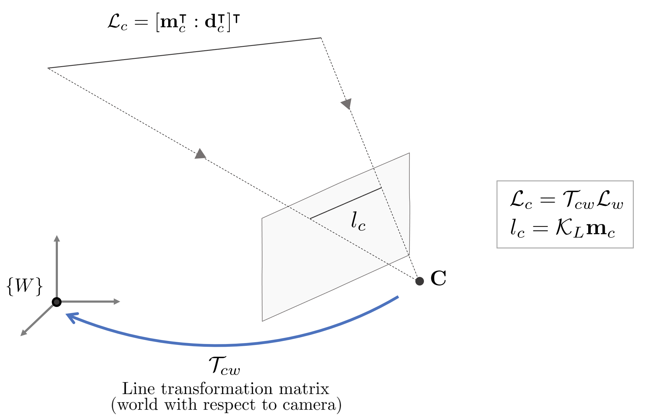
3차원 공간 상의 직선은 Plücker Coordinate를 사용하여 6차원 열벡터로 표현할 수 있다. 

$$\begin{array}{}\text{(130)}& \begin{array}{rl}\mathcal{L}& =[{\mathbf{m}}^{⊺}:{\mathbf{d}}^{⊺}{]}^{⊺}=[m_x:m_y:m_z:d_x:d_y:d_z{]}^{⊺}\end{array}\end{array}$$

 

앞서 설명한 $[\mathbf{d}:\mathbf{m}]$ 순서와 달리 Plücker Coordinate를 활용한 논문에서는 대부분 $[\mathbf{m}:\mathbf{d}]$ 순서를 사용하기 때문에 본 섹션에서도 해당 순서로 직선을 표현한다. 해당 직선 표현법은 스케일 모호성을 가지고 있기 때문에(up to scale) 5자유도를 가지며 $\mathbf{m},\mathbf{d}$은 단위 벡터가 아니어도 두 벡터 값의 비율에 의해 직선을 유일하게 표현할 수 있다.

 

6.1. Line Transformation and projection

월드 좌표계에서 본 직선을 ${\mathcal{L}}_w$라고 하면 이를 카메라 좌표계에서 봤을 경우 다음과 같이 변환할 수 있다. 

$$\begin{array}{}\text{(131)}& \begin{array}{rl}{\mathcal{L}}_c& =\left[\begin{array}{c}{\mathbf{m}}_c\\ {\mathbf{d}}_c\end{array}\right]={\mathcal{T}}_{cw}{\mathcal{L}}_w=\left[\begin{array}{cc}{\mathbf{R}}_{cw}& {\mathbf{t}}^{\wedge }{\mathbf{R}}_{cw}\\ 0& {\mathbf{R}}_{cw}\end{array}\right]\left[\begin{array}{c}{\mathbf{m}}_w\\ {\mathbf{d}}_w\end{array}\right]\end{array}\end{array}$$

 

해당 직선을 이미지 평면 상에 프로젝션시키면 다음과 같다.

$$\begin{array}{}\text{(132)}& \begin{array}{rl}{l}_c& =\left[\begin{array}{c}{l}_1\\ l_2\\ l_3\end{array}\right]={\mathcal{K}}_L{\mathbf{m}}_c=\left[\begin{array}{ccc}{f}_y& & \\ & f_x& \\ -f_y{c}_x& -f_x{c}_y& f_x{f}_y\end{array}\right]\left[\begin{array}{c}{m}_x\\ m_y\\ m_z\end{array}\right]\end{array}\end{array}$$

 

${\mathcal{K}}_L$는 $\mathcal{P}=[det(\mathbf{N}){\mathbf{N}}^{-⊺}|{\mathbf{n}}^{\wedge }\mathbf{N}]$에서 $\mathbf{P}=K[\mathbf{I}|\mathbf{0}]$인 경우를 의미한다. 따라서 $\mathcal{P}=[det(\mathbf{K}){\mathbf{K}}^{-⊺}|\mathbf{0}]$이 되므로 $\mathcal{L}$의 $\mathbf{d}$ 항이 0으로 소거된다. 따라서 $\mathbf{K}=\left[\begin{array}{ccc}{f}_x& & c_x\\ & f_y& c_y\\ & & 1\end{array}\right]$ 일 때 다음과 같은 식이 유도된다.

$$\begin{array}{}\text{(133)}& \begin{array}{r}{\mathcal{K}}_L=det(\mathbf{K}){\mathbf{K}}^{-⊺}=\left[\begin{array}{ccc}{f}_y& & \\ & f_x& \\ -f_y{c}_x& -f_x{c}_y& f_x{f}_y\end{array}\right]\in {\mathbb{R}}^{3\times 3}\end{array}\end{array}$$

 

6.2. Line reprojection error

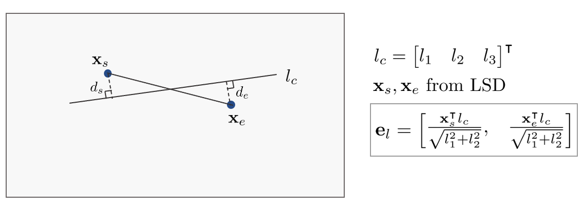
직선의 reprojection 에러 ${\mathbf{e}}_l$은 다음과 같이 나타낼 수 있다.

$$\begin{array}{}\text{(134)}& \begin{array}{r}{\mathbf{e}}_l=\left[\begin{array}{c}{d}_s,d_e\end{array}\right]=\left[\begin{array}{cc}\frac{{\mathbf{x}}_s^{⊺}{l}_c}{\sqrt{l_1^2+l_2^2}},& \frac{{\mathbf{x}}_e^{⊺}{l}_c}{\sqrt{l_1^2+l_2^2}}\end{array}\right]\in {\mathbb{R}}^2\end{array}\end{array}$$

 

이는 점과 직선 사이의 거리  공식을 통해 나타낼 수 있다. 이 때, $\{{\mathbf{x}}_s,{\mathbf{x}}_e\}$는 각각 line feature extracture(e.g., LSD)를 사용하여 추출한 직선의 시작점과 끝점을 의미한다.  즉, ${\mathcal{l}}_c$가 모델링을 통해 구한 예측값이고 ${\mathbf{x}}_s,{\mathbf{x}}_e$를 잇는 직선이 센서 데이터를 통해 측정한 관측값이 된다.

 

6.3. Orthonormal representation

앞서 구한 ${\mathbf{e}}_l$를 사용하여 BA 최적화를 수행할 때 Plücker Coordinate 표현법을 그대로 사용하게 되면 문제가 발생한다.  Plücker Coordinate는 항상 ${\mathbf{m}}^{⊺}\mathbf{d}=0$이라는 Klein quadric 제약조건을 만족해야 하기 때문에 5자유도를 가지므로 직선을 표현할 수 있는 최소 파라미터 개수인 4개의 비해 over-parameterized 되어 있다. Over-parameterized된 표현법의 단점은 다음과 같다.

• 중복되는 파라미터를 계산해야 하기 때문에 최적화 수행 시 연산량이 증가한다.
• 추가적인 자유도로 인해 수치적인 불안정성(numerical instability) 문제가 야기될 수 있다.
• 파라미터가 업데이트될 때마다 항상 제약조건을 만족하는 지 체크해줘야 한다.

 

따라서 직선을 최적화 할 때는 일반적으로 최소 파라미터인 4자유도로 변경하기 위해 orthonormal 표현법을 사용한다. 즉, 직선을 표현할 때는 Plücker Coordinate를 사용하지만 최적화를 수행할 때는 orthonormal 표현법으로 변형한 뒤 최적값을 업데이트하고 다시 Plücker Coordinate로 돌아오는 방식을 취한다.

 

Orthonormal 표현법은 다음과 같다. 3차원 공간 상의 직선은 항상 다음과 같이 표현 가능하다.

$$\begin{array}{}\text{(135)}& \begin{array}{r}(\mathbf{U},\mathbf{W})\in SO(3)\times SO(2)\end{array}\end{array}$$

 

임의의 Plücker 직선 $\mathcal{L}=[{\mathbf{m}}^{⊺}:{\mathbf{d}}^{⊺}{]}^{⊺}$은 이와 일대일 대응하는 $(\mathbf{U},\mathbf{W})$를 항상 가지고 있으며 이러한 표현 방법을 orthonormal 표현법이라고 한다. 월드 상의 한 직선 ${\mathcal{L}}_w=[{\mathbf{m}}_w^{⊺}:{\mathbf{d}}_w^{⊺}{]}^{⊺}$이 주어졌을 때 ${\mathcal{L}}_w$을 QR decomposition 함으로써 $(\mathbf{U},\mathbf{W})$구할 수 있다.

$$\begin{array}{}\text{(136)}& \begin{array}{r}\left[\begin{array}{c}{\mathbf{m}}_w|{\mathbf{d}}_w\end{array}\right]=\mathbf{U}\left[\begin{array}{cc}{w}_1& 0\\ 0& w_2\\ 0& 0\end{array}\right],\text{with set: }\mathbf{W}=\left[\begin{array}{cc}{w}_1& -w_2\\ w_2& w_1\end{array}\right]\end{array}\end{array}$$

 

이 때, 상삼각행렬(upper triangle matrix) $\mathbf{R}$의 $(1,2)$ 원소는 Plücker 제약조건(Klein quadric)으로 인해 항상 0이 된다. $\mathbf{U},\mathbf{W}$는 각각 3차원, 2차원 회전행렬을 의미하므로 $\mathbf{U}=\mathbf{R}(\mathit{\theta }),\mathbf{W}=\mathbf{R}(\theta )$와 같이 나타낼 수 있다. 

$$\begin{array}{}\text{(137)}& \begin{array}{rl}\mathbf{R}(\mathit{\theta })& =\mathbf{U}=\left[\begin{array}{ccc}{\mathbf{u}}_1& {\mathbf{u}}_2& {\mathbf{u}}_3\end{array}\right]=\left[\begin{array}{ccc}\frac{{\mathbf{m}}_w}{\Vert {\mathbf{m}}_w\Vert }& \frac{{\mathbf{d}}_w}{\Vert {\mathbf{d}}_w\Vert }& \frac{{\mathbf{m}}_w\times {\mathbf{d}}_w}{\Vert {\mathbf{m}}_w\times {\mathbf{d}}_w\Vert }\end{array}\right]\\ \mathbf{R}(\theta )& =\mathbf{W}=\left[\begin{array}{cc}{w}_1& -w_2\\ w_2& w_1\end{array}\right]=\left[\begin{array}{cc}\cos \theta & -\sin \theta \\ \sin \theta & \cos \theta \end{array}\right]\\ & =\frac{1}{\sqrt{{\Vert {\mathbf{m}}_w\Vert }^2+{\Vert {\mathbf{d}}_w\Vert }^2}}\left[\begin{array}{cc}\Vert {\mathbf{m}}_w\Vert & \Vert {\mathbf{d}}_w\Vert \\ -\Vert {\mathbf{d}}_w\Vert & \Vert {\mathbf{m}}_w\Vert \end{array}\right]\end{array}\end{array}$$

 

실제 최적화를 수행할 때는 $\mathbf{U}\leftarrow \mathbf{U}\mathbf{R}(\mathit{\theta }),\mathbf{W}\leftarrow \mathbf{W}\mathbf{R}(\theta )$과 같이 업데이트된다. 따라서 orthonormal 표현법은 3차원 공간 상의 직선을 ${\delta }_{\mathit{\theta }}=[{\mathit{\theta }}^{⊺},\theta ]\in {\mathbb{R}}^4$를 통해 4자유도로 표현할 수 있다. 최적화를 통해 업데이트된 $[{\mathit{\theta }}^{⊺},\theta ]$는 다음과 같이 ${\mathcal{L}}_w$로 변환된다.

$$\begin{array}{}\text{(138)}& \begin{array}{r}{\mathcal{L}}_w=\left[\begin{array}{cc}{w}_1{\mathbf{u}}_1^{⊺}& w_2{\mathbf{u}}_2^{⊺}\end{array}\right]\end{array}\end{array}$$

 

6.4. Error function formulation

직선에 대한 reprojection 에러 ${\mathbf{e}}_l$를 최적화하기 위해서는 Gauss-Newton(GN), Levenberg-Marquardt(LM) 등의 비선형 최소제곱법을 사용하여 반복적으로(iterative) 최적 변수를 업데이트해야 한다. reprojection 에러를 사용하여 에러 함수를 표현하면 다음과 같다.

$$\begin{array}{}\text{(139)}& \begin{array}{rl}{\mathbf{E}}_l(\mathcal{X})& =\sum _i\sum _j{\Vert {\mathbf{e}}_{l,ij}\Vert }^2\end{array}\end{array}$$
$$\begin{array}{}\text{(140)}& \begin{array}{rl}{\mathcal{X}}^{\ast }& =\arg \underset{{\mathcal{X}}^{\ast }}{min}{\mathbf{E}}_l(\mathcal{X})\\ & =\arg \underset{{\mathcal{X}}^{\ast }}{min}\sum _i\sum _j{\Vert {\mathbf{e}}_{l,ij}\Vert }^2\\ & =\arg \underset{{\mathcal{X}}^{\ast }}{min}\sum _i\sum _j{\mathbf{e}}_{l,ij}^{⊺}{\mathbf{e}}_{l,ij}\end{array}\end{array}$$

 

${\mathbf{E}}_l({\mathcal{X}}^{\ast })$를 만족하는 ${\Vert {\mathbf{e}}_l({\mathcal{X}}^{\ast })\Vert }^2$를 non-linear least squares를 통해 반복적으로 계산할 수 있다. 작은 증분량 $\mathrm{\Delta }\mathcal{X}$를 반복적으로 $\mathcal{X}$에 업데이트함으로써 최적의 상태를 찾는다. 
$$\begin{array}{}\text{(141)}& \begin{array}{rl}\arg \underset{{\mathcal{X}}^{\ast }}{min}{\mathbf{E}}_l(\mathcal{X}+\mathrm{\Delta }\mathcal{X})& =\arg \underset{{\mathcal{X}}^{\ast }}{min}\sum _i\sum _j{\Vert {\mathbf{e}}_l(\mathcal{X}+\mathrm{\Delta }\mathcal{X})\Vert }^2\end{array}\end{array}$$

엄밀하게 말하면 상태 증분량 $\mathrm{\Delta }\mathcal{X}$은 SE(3) 변환행렬을 포함하므로 $\oplus$ 연산자를 통해 기존 상태 $\mathcal{X}$에 더해지는게 맞지만 표현의 편의를 위해 $+$ 연산자를 사용하였다.

$$\begin{array}{}\text{(142)}& \begin{array}{r}{\mathbf{e}}_l(\mathcal{X}\oplus \mathrm{\Delta }\mathcal{X})\to {\mathbf{e}}_l(\mathcal{X}+\mathrm{\Delta }\mathcal{X})\end{array}\end{array}$$

 

위 식은 테일러 1차 근사를 통해 다음과 같이 표현이 가능하다.
$$\begin{array}{}\text{(143)}& \begin{array}{rl}{\mathbf{e}}_l(\mathcal{X}+\mathrm{\Delta }\mathcal{X})& \approx {\mathbf{e}}_l(\mathcal{X})+\mathbf{J}\mathrm{\Delta }\mathcal{X}\\ & ={\mathbf{e}}_l(\mathcal{X})+{\mathbf{J}}_{\mathit{\theta }}\mathrm{\Delta }{\delta }_{\mathit{\theta }}+{\mathbf{J}}_{\xi }\mathrm{\Delta }{\delta }_{\xi }\\ & ={\mathbf{e}}_l(\mathcal{X})+\frac{\partial {\mathbf{e}}_l}{\partial {\delta }_{\mathit{\theta }}}\mathrm{\Delta }{\delta }_{\mathit{\theta }}+\frac{\partial {\mathbf{e}}_l}{\partial {\delta }_{\xi }}\mathrm{\Delta }{\delta }_{\xi }\end{array}\end{array}$$

 

$$\begin{array}{}\text{(144)}& \begin{array}{rl}\arg \underset{{\mathcal{X}}^{\ast }}{min}{\mathbf{E}}_l(\mathcal{X}+\mathrm{\Delta }\mathcal{X})& \approx \arg \underset{{\mathcal{X}}^{\ast }}{min}\sum _i\sum _j{\Vert {\mathbf{e}}_l(\mathcal{X})+\mathbf{J}\mathrm{\Delta }\mathcal{X}\Vert }^2\end{array}\end{array}$$

 

이를 미분하여 최적의 증분량 $\mathrm{\Delta }{\mathcal{X}}^{\ast }$ 값을 구하면 다음과 같다. 자세한 유도 과정은 본 섹션에서는 생략한다. 유도 과정에 대해 자세히 알고 싶으면 이전 섹션을 참조하면 된다.
$$\begin{array}{}\text{(145)}& \begin{array}{rl}& {\mathbf{J}}^{⊺}\mathbf{J}\mathrm{\Delta }{\mathcal{X}}^{\ast }=-{\mathbf{J}}^{⊺}\mathbf{e}\\ & \mathbf{H}\mathrm{\Delta }{\mathcal{X}}^{\ast }=-\mathbf{b}\end{array}\end{array}$$

 

6.4.1. The analytical jacobian of 3d line

이전 섹션에서 설명한 것처럼 비선형 최적화를 수행하기 위해서는 $\mathbf{J}$를 계산해야 한다. $\mathbf{J}$는 다음과 같이 구성되어 있다.

$$\begin{array}{}\text{(146)}& \begin{array}{rl}& \mathbf{J}=[{\mathbf{J}}_{\mathit{\theta }},{\mathbf{J}}_{\xi }]\end{array}\end{array}$$

 

$[{\mathbf{J}}_{\mathit{\theta }},{\mathbf{J}}_{\xi }]$는 다음과 같이 전개할 수 있다.

$$\begin{array}{}\text{(147)}& \begin{array}{rl}& {\mathbf{J}}_{\mathit{\theta }}=\frac{\partial {\mathbf{e}}_l}{\partial {\delta }_{\mathit{\theta }}}=\frac{\partial {\mathbf{e}}_l}{\partial l}\frac{\partial l}{\partial {\mathcal{L}}_c}\frac{\partial {\mathcal{L}}_c}{\partial {\mathcal{L}}_w}\frac{\partial {\mathcal{L}}_w}{\partial {\delta }_{\mathit{\theta }}}\\ & {\mathbf{J}}_{\xi }=\frac{\partial {\mathbf{e}}_l}{\partial {\delta }_{\xi }}=\frac{\partial {\mathbf{e}}_l}{\partial l}\frac{\partial l}{\partial {\mathcal{L}}_c}\frac{\partial {\mathcal{L}}_c}{\partial {\delta }_{\xi }}\end{array}\end{array}$$

 

$\frac{\partial {\mathbf{e}}_l}{\partial l}$는 다음과 같이 구할 수 있다. 이 때, $l$은 벡터이고 $l_i$는 스칼라임에 유의한다.

$$\begin{array}{}\text{(148)}& \boxed{{\displaystyle \begin{array}{r}\frac{\partial {\mathbf{e}}_l}{\partial l}=\frac{1}{\sqrt{l_1^2+l_2^2}}\left[\begin{array}{ccc}{x}_s-\frac{l_1{\mathbf{x}}_{s}l}{\sqrt{l_1^2+l_2^2}}& y_s-\frac{l_2{\mathbf{x}}_{s}l}{\sqrt{l_1^2+l_2^2}}& 1\\ x_e-\frac{l_1{\mathbf{x}}_{e}l}{\sqrt{l_1^2+l_2^2}}& y_e-\frac{l_2{\mathbf{x}}_{e}l}{\sqrt{l_1^2+l_2^2}}& 1\end{array}\right]\in {\mathbb{R}}^{2\times 3}\end{array}}}\end{array}$$

 

$\frac{\partial l}{\partial {\mathcal{L}}_c}$는 다음과 같이 구할 수 있다.

$$\begin{array}{}\text{(149)}& \boxed{{\displaystyle \begin{array}{r}\frac{\partial l}{\partial {\mathcal{L}}_c}=\frac{\partial {\mathcal{K}}_L{\mathbf{m}}_c}{\partial {\mathcal{L}}_c}=\left[\begin{array}{cc}{\mathcal{K}}_L& {\mathbf{0}}_{3\times 3}\end{array}\right]=\left[\begin{array}{cccccc}{f}_y& & & 0& 0& 0\\ & f_x& & 0& 0& 0\\ -f_y{c}_x& -f_x{c}_y& f_x{f}_y& 0& 0& 0\end{array}\right]\in {\mathbb{R}}^{3\times 6}\end{array}}}\end{array}$$

 

$\frac{\partial {\mathcal{L}}_c}{\partial {\mathcal{L}}_w}$는 다음과 같이 구할 수 있다.

$$\begin{array}{}\text{(150)}& \boxed{{\displaystyle \begin{array}{r}\frac{\partial {\mathcal{L}}_c}{\partial {\mathcal{L}}_w}=\frac{\partial {\mathcal{T}}_{cw}{\mathcal{L}}_w}{\partial {\mathcal{L}}_w}={\mathcal{T}}_{cw}=\left[\begin{array}{cc}{\mathbf{R}}_{cw}& {\mathbf{t}}^{\wedge }{\mathbf{R}}_{cw}\\ 0& {\mathbf{R}}_{cw}\end{array}\right]\in {\mathbb{R}}^{6\times 6}\end{array}}}\end{array}$$

 

orthonormal 표현법에 대한 자코비안 $\frac{\partial {\mathcal{L}}_w}{\partial {\delta }_{\mathit{\theta }}}$는 다음과 같이 구할 수 있다.

$$\begin{array}{}\text{(151)}& \boxed{{\displaystyle \begin{array}{r}\frac{\partial {\mathcal{L}}_w}{\partial {\delta }_{\mathit{\theta }}}=\left[\begin{array}{cccc}{\mathbf{0}}_{3\times 1}& -w_1{\mathbf{u}}_3& w_1{\mathbf{u}}_2& -w_2{\mathbf{u}}_1\\ w_2{\mathbf{u}}_3& {\mathbf{0}}_{3\times 1}& -w_2{\mathbf{u}}_1& w_1{\mathbf{u}}_2\end{array}\right]\in {\mathbb{R}}^{6\times 4}\end{array}}}\end{array}$$

 

카메라 포즈에 대한 자코비안 $\frac{\partial {\mathcal{L}}_c}{\partial {\delta }_{\xi }}$는 다음과 같이 구할 수 있다.

$$\begin{array}{}\text{(152)}& \boxed{{\displaystyle \begin{array}{r}\frac{\partial {\mathcal{L}}_c}{\partial {\delta }_{\xi }}=\left[\begin{array}{cc}-(\mathbf{R}\mathbf{m}{)}^{\wedge }-({\mathbf{t}}^{\wedge }\mathbf{Rd}{)}^{\wedge }& -(\mathbf{Rd}{)}^{\wedge }\\ -(\mathbf{Rd}{)}^{\wedge }& {\mathbf{0}}_{3\times 3}\end{array}\right]\in {\mathbb{R}}^{6\times 6}\end{array}}}\end{array}$$

 

6.5. Code implementations

• Structure PLP SLAM 코드: g2o/se3/pose_opt_edge_line3d_orthonormal.h#L62
• Structure PLP SLAM 코드2: g2o/se3/pose_opt_edge_line3d_orthonormal.h#L81